Diffusion for Audio
In this notebook, we’re going to take a brief look at generating audio with diffusion models.
What you will learn:
- How audio is represented in a computer
- Methods to convert between raw audio data and spectrograms
- How to prepare a dataloader with a custom collate function to convert audio slices into spectrograms
- Fine-tuning an existing audio diffusion model on a specific genre of music
- Uploading your custom pipeline to the Hugging Face hub
Caveat: This is mostly for educational purposes - no guarantees our model will sound good 😉.
Let’s get started!
Setup and Imports
%pip install -q datasets diffusers torchaudio accelerate
import torch, random
import numpy as np
import torch.nn.functional as F
from tqdm.auto import tqdm
from IPython.display import Audio
from matplotlib import pyplot as plt
from diffusers import DiffusionPipeline
from torchaudio import transforms as AT
from torchvision import transforms as IT
Sampling from a Pre-Trained Audio Pipeline
Let’s begin by following the Audio Diffusion docs to load a pre-existing audio diffusion model pipeline:
# Load a pre-trained audio diffusion pipeline
device = "mps" if torch.backends.mps.is_available() else "cuda" if torch.cuda.is_available() else "cpu"
pipe = DiffusionPipeline.from_pretrained("teticio/audio-diffusion-instrumental-hiphop-256").to(device)
As with the pipelines we’ve used in previous units, we can create samples by calling the pipeline like so:
>>> # Sample from the pipeline and display the outputs
>>> output = pipe()
>>> display(output.images[0])
>>> display(Audio(output.audios[0], rate=pipe.mel.get_sample_rate()))
Here, the rate argument specifies the sampling rate for the audio; we’ll take a deeper look at this later. You’ll also notice there are multiple things returned by the pipeline. What’s going on here? Let’s take a closer look at both outputs.
The first is an array of data, representing the generated audio:
# The audio array
output.audios[0].shape
The second looks like a greyscale image:
# The output image (spectrogram)
output.images[0].size
This gives us a hint at how this pipeline works. The audio is not directly generated with diffusion - instead, the pipeline has the same kind of 2D UNet as the unconditional image generation pipelines we saw in Unit 1 that is used to generate the spectrogram, which is then post-processed into the final audio.
The pipe has an extra component that handles these conversions, which we can access via pipe.mel:
pipe.mel
From Audio to Image and Back Again
An audio ‘waveform’ encodes the raw audio samples over time - this could be the electrical signal received from a microphone, for example. Working with this ‘Time Domain’ representation can be tricky, so it is a common practice to convert it into some other form, commonly something called a spectrogram. A spectrogram shows the intensity of different frequencies (y axis) vs time (x axis):
>>> # Calculate and show a spectrogram for our generated audio sample using torchaudio
>>> spec_transform = AT.Spectrogram(power=2)
>>> spectrogram = spec_transform(torch.tensor(output.audios[0]))
>>> print(spectrogram.min(), spectrogram.max())
>>> log_spectrogram = spectrogram.log()
>>> plt.imshow(log_spectrogram[0], cmap="gray")
tensor(0.) tensor(6.0842)
The spectrogram we just made has values between 0.0000000000001 and 1, with most being close to the low end of that range. This is not ideal for visualization or modelling - in fact we had to take the log of these values to get a greyscale plot that showed any detail. For this reason, we typically use a special kind of spectrogram called a Mel spectrogram, which is designed to capture the kinds of information which are important for human hearing by applying some transforms to the different frequency components of the signal.
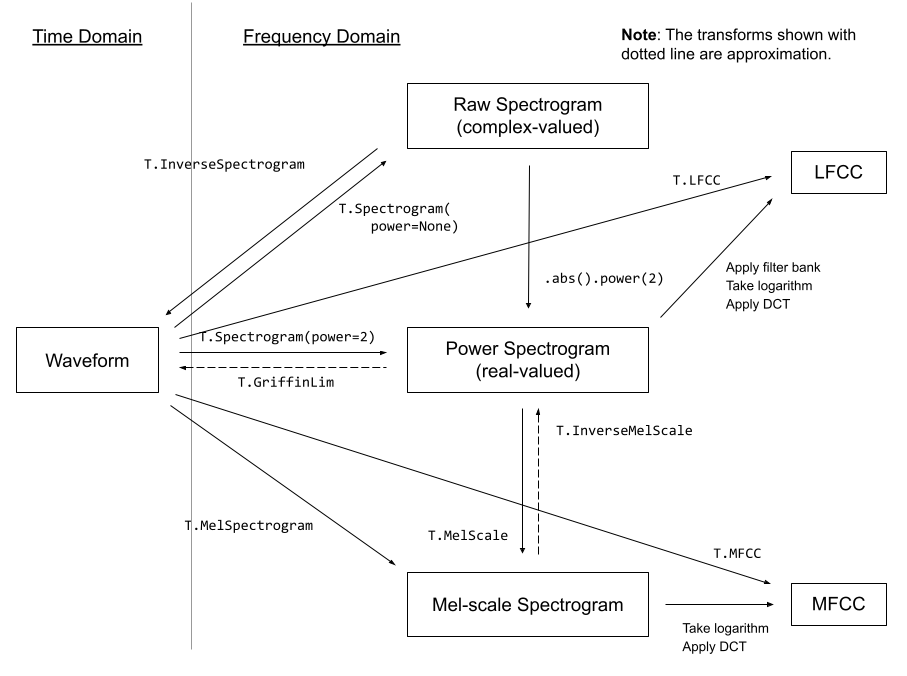 Some audio transforms from the torchaudio docs
Luckily for us, we don’t even need to worry too much about these transforms - the pipeline’s mel functionality handles these details for us. Using this, we can convert a spectrogram image to audio like so:
a = pipe.mel.image_to_audio(output.images[0])
a.shape
And we can convert an array of audio data into a spectrogram images by first loading the raw audio data and then calling the audio_slice_to_image() function. Longer clips are automatically sliced into chunks of the correct length to produce a 256x256 spectrogram image:
>>> pipe.mel.load_audio(raw_audio=a)
>>> im = pipe.mel.audio_slice_to_image(0)
>>> im
The audio is represented as a long array of numbers. To play this out loud we need one more key piece of information: the sample rate. How many samples (individual values) do we use to represent a single second of audio?
We can see the sample rate used during training of this pipeline with:
sample_rate_pipeline = pipe.mel.get_sample_rate()
sample_rate_pipeline
If we specify the sample rate incorrectly, we get audio that is sped up or slowed down:
display(Audio(output.audios[0], rate=44100)) # 2x speedFine-Tuning the pipeline
Now that we have a rough understanding of how the pipeline works, let’s fine-tune it on some new audio data!
The dataset is a collection of audio clips in different genres, which we can load from the hub like so:
from datasets import load_dataset

dataset = load_dataset("lewtun/music_genres", split="train")
dataset
You can use the code below to see the different genres in the dataset and how many samples are contained in each:
>>> for g in list(set(dataset["genre"])):
...     print(g, sum(x == g for x in dataset["genre"]))
Pop 945 Blues 58 Punk 2582 Old-Time / Historic 408 Experimental 1800 Folk 1214 Electronic 3071 Spoken 94 Classical 495 Country 142 Instrumental 1044 Chiptune / Glitch 1181 International 814 Ambient Electronic 796 Jazz 306 Soul-RnB 94 Hip-Hop 1757 Easy Listening 13 Rock 3095
The dataset has the audio as arrays:
>>> audio_array = dataset[0]["audio"]["array"]
>>> sample_rate_dataset = dataset[0]["audio"]["sampling_rate"]
>>> print("Audio array shape:", audio_array.shape)
>>> print("Sample rate:", sample_rate_dataset)
>>> display(Audio(audio_array, rate=sample_rate_dataset))
Audio array shape: (1323119,) Sample rate: 44100
Note that the sample rate of this audio is higher - if we want to use the existing pipeline we’ll need to ‘resample’ it to match. The clips are also longer than the ones the pipeline is set up for. Fortunately, when we load the audio using pipe.mel it automatically slices the clip into smaller sections:
>>> a = dataset[0]["audio"]["array"]  # Get the audio array
>>> pipe.mel.load_audio(raw_audio=a)  # Load it with pipe.mel
>>> pipe.mel.audio_slice_to_image(0)  # View the first 'slice' as a spectrogram
We need to remember to adjust the sampling rate, since the data from this dataset has twice as many samples per second:
sample_rate_dataset = dataset[0]["audio"]["sampling_rate"]
sample_rate_dataset
Here we use torchaudio’s transforms (imported as AT) to do the resampling, the pipe’s mel to turn audio into an image and torchvision’s transforms (imported as IT) to turn images into tensors. This gives us a function that turns an audio clip into a spectrogram tensor that we can use for training:
resampler = AT.Resample(sample_rate_dataset, sample_rate_pipeline, dtype=torch.float32)
to_t = IT.ToTensor()


def to_image(audio_array):
    audio_tensor = torch.tensor(audio_array).to(torch.float32)
    audio_tensor = resampler(audio_tensor)
    pipe.mel.load_audio(raw_audio=np.array(audio_tensor))
    num_slices = pipe.mel.get_number_of_slices()
    slice_idx = random.randint(0, num_slices - 1)  # Pic a random slice each time (excluding the last short slice)
    im = pipe.mel.audio_slice_to_image(slice_idx)
    return im
We’ll use our to_image() function as part of a custom collate function to turn our dataset into a dataloader we can use for training. The collate function defines how to transform a batch of examples from the dataset into the final batch of data ready for training. In this case we turn each audio sample into a spectrogram image and stack the resulting tensors together:
>>> def collate_fn(examples):
...     # to image -> to tensor -> rescale to (-1, 1) -> stack into batch
...     audio_ims = [to_t(to_image(x["audio"]["array"])) * 2 - 1 for x in examples]
...     return torch.stack(audio_ims)


>>> # Create a dataset with only the 'Chiptune / Glitch' genre of songs
>>> batch_size = 4  # 4 on colab, 12 on A100
>>> chosen_genre = "Electronic"  # <<< Try training on different genres <<<
>>> indexes = [i for i, g in enumerate(dataset["genre"]) if g == chosen_genre]
>>> filtered_dataset = dataset.select(indexes)
>>> dl = torch.utils.data.DataLoader(
...     filtered_dataset.shuffle(), batch_size=batch_size, collate_fn=collate_fn, shuffle=True
... )
>>> batch = next(iter(dl))
>>> print(batch.shape)
torch.Size([4, 1, 256, 256])
NB: You will need to use a lower batch size (e.g., 4) unless you have plenty of GPU vRAM available.
Training Loop
Here is a simple training loop that runs through the dataloader for a few epochs to fine-tune the pipeline’s UNet. You can also skip this cell and load the pipeline with the code in the following cell.
epochs = 3
lr = 1e-4

pipe.unet.train()
pipe.scheduler.set_timesteps(1000)
optimizer = torch.optim.AdamW(pipe.unet.parameters(), lr=lr)

for epoch in range(epochs):
    for step, batch in tqdm(enumerate(dl), total=len(dl)):

        # Prepare the input images
        clean_images = batch.to(device)
        bs = clean_images.shape[0]

        # Sample a random timestep for each image
        timesteps = torch.randint(0, pipe.scheduler.num_train_timesteps, (bs,), device=clean_images.device).long()

        # Add noise to the clean images according to the noise magnitude at each timestep
        noise = torch.randn(clean_images.shape).to(clean_images.device)
        noisy_images = pipe.scheduler.add_noise(clean_images, noise, timesteps)

        # Get the model prediction
        noise_pred = pipe.unet(noisy_images, timesteps, return_dict=False)[0]

        # Calculate the loss
        loss = F.mse_loss(noise_pred, noise)
        loss.backward(loss)

        # Update the model parameters with the optimizer
        optimizer.step()
optimizer.zero_grad()# OR: Load the version I trained earlier
pipe = DiffusionPipeline.from_pretrained("johnowhitaker/Electronic_test").to(device)>>> output = pipe()
>>> display(output.images[0])
>>> display(Audio(output.audios[0], rate=22050))
>>> # Make a longer sample by passing in a starting noise tensor with a different shape
>>> noise = torch.randn(1, 1, pipe.unet.sample_size[0], pipe.unet.sample_size[1] * 4).to(device)
>>> output = pipe(noise=noise)
>>> display(output.images[0])
>>> display(Audio(output.audios[0], rate=22050))
Not the most amazing-sounding outputs, but it’s a start :) Explore tweaking the learning rate and number of epochs, and share your best results on Discord so we can improve together!
Some things to consider:
- We’re working with 256px square spectrogram images which limits our batch size. Can you recover audio of sufficient quality from a 128x128 spectrogram?
- In place of random image augmentation we’re picking different slices of the audio clip each time, but could this be improved with some different kinds of augmentation when training for many epochs?
- How else might we use this to generate longer clips? Perhaps you could generate a 5s starting clip and then use inpainting-inspired ideas to continue to generate additional segments of audio that follow on from the initial clip…
- What is the equivalent of image-to-image in this spectrogram diffusion context?
Push to Hub
Once you’re happy with your model, you can save it and push it to the hub for others to enjoy:
from huggingface_hub import get_full_repo_name, HfApi, create_repo, ModelCard# Pick a name for the model
model_name = "audio-diffusion-electronic"
hub_model_id = get_full_repo_name(model_name)# Save the pipeline locally
pipe.save_pretrained(model_name)>>> # Inspect the folder contents
>>> !ls {model_name}mel model_index.json scheduler unet
# Create a repository
create_repo(hub_model_id)# Upload the files
api = HfApi()
api.upload_folder(folder_path=f"{model_name}/scheduler", path_in_repo="scheduler", repo_id=hub_model_id)
api.upload_folder(folder_path=f"{model_name}/mel", path_in_repo="mel", repo_id=hub_model_id)
api.upload_folder(folder_path=f"{model_name}/unet", path_in_repo="unet", repo_id=hub_model_id)
api.upload_file(
path_or_fileobj=f"{model_name}/model_index.json",
path_in_repo="model_index.json",
repo_id=hub_model_id,
)# Push a model card
content = f"""
---
license: mit
tags:
- pytorch
- diffusers
- unconditional-audio-generation
- diffusion-models-class
---
# Model Card for Unit 4 of the [Diffusion Models Class 🧨](https://github.com/huggingface/diffusion-models-class)
This model is a diffusion model for unconditional audio generation of music in the genre {chosen_genre}
## Usage
<pre>
from IPython.display import Audio
from diffusers import DiffusionPipeline
pipe = DiffusionPipeline.from_pretrained("{hub_model_id}")
output = pipe()
display(output.images[0])
display(Audio(output.audios[0], rate=pipe.mel.get_sample_rate()))
</pre>
"""
card = ModelCard(content)
card.push_to_hub(hub_model_id)Conclusion
This notebook has hopefully given you a small taste of the potential of audio generation. Check out some of the references linked from the introduction to this unit to see some fancier methods and the astounding samples they can create!