History of State Space Models (SSM) in 2022

Introduction

In the previous article, we defined a State Space Model (SSM) using a continuous-time system. We discretized it to show its recurrent and then convolutive view. The interest here is in being able to train the model convolutely and then perform inference recursively over very long sequences.

Figure 1: Image from blog post « Structured State Spaces: Combining Continuous-Time, Recurrent, and Convolutional Models » by Albert GU et al. (2022)

This vision was introduced by Albert GU in his papers LSSL and S4 published in 2021. S4 being the equivalent of "Attention is all you need" for transformers.
In this article, we will review the SSM literature published in 2022. Those appearing in 2023 will be listed in the next article. The aim is to show the different evolutions of these types of models over the months, while remaining synthetic (i.e. I won't go into all the details of the papers listed). During this year 2022, the various advances have focused on applying different discretization algorithms, while replacing the HiPPO matrix with a simpler one.

Theoretical models

In this section, we will review the theoretical work behind the proposed improvements to the S4 architecture. Then, in a different section, we'll look at concrete applications to different tasks (audio, vision, etc.).

S4 V2

On March 4, 2022, the authors of S4 updated their paper to include a section on the importance of the HiPPO matrix (see section 4.4 of the most recent version of the paper).
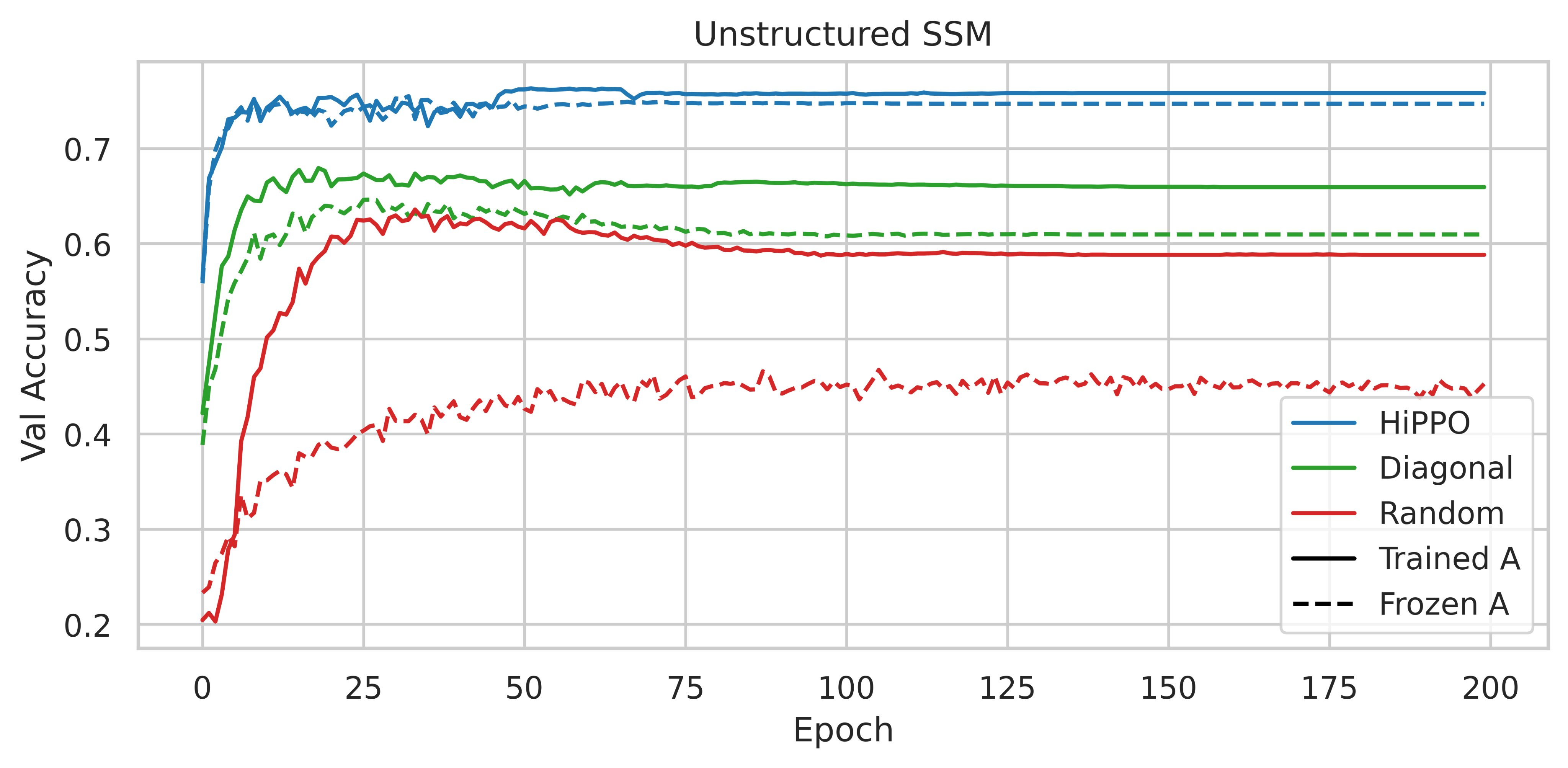
In a nutshell, it consists in reporting the results observed following the performance of ablations on the CIFAR-10 sequential dataset. Instead of using an SSM with the HiPPO matrix, the authors have tried to use various parameterizations such as a random dense matrix and a random diagonal matrix.

Figure 2: Accuracy on the CIFAR-10 validation split, from figure 3 of the S4 paper

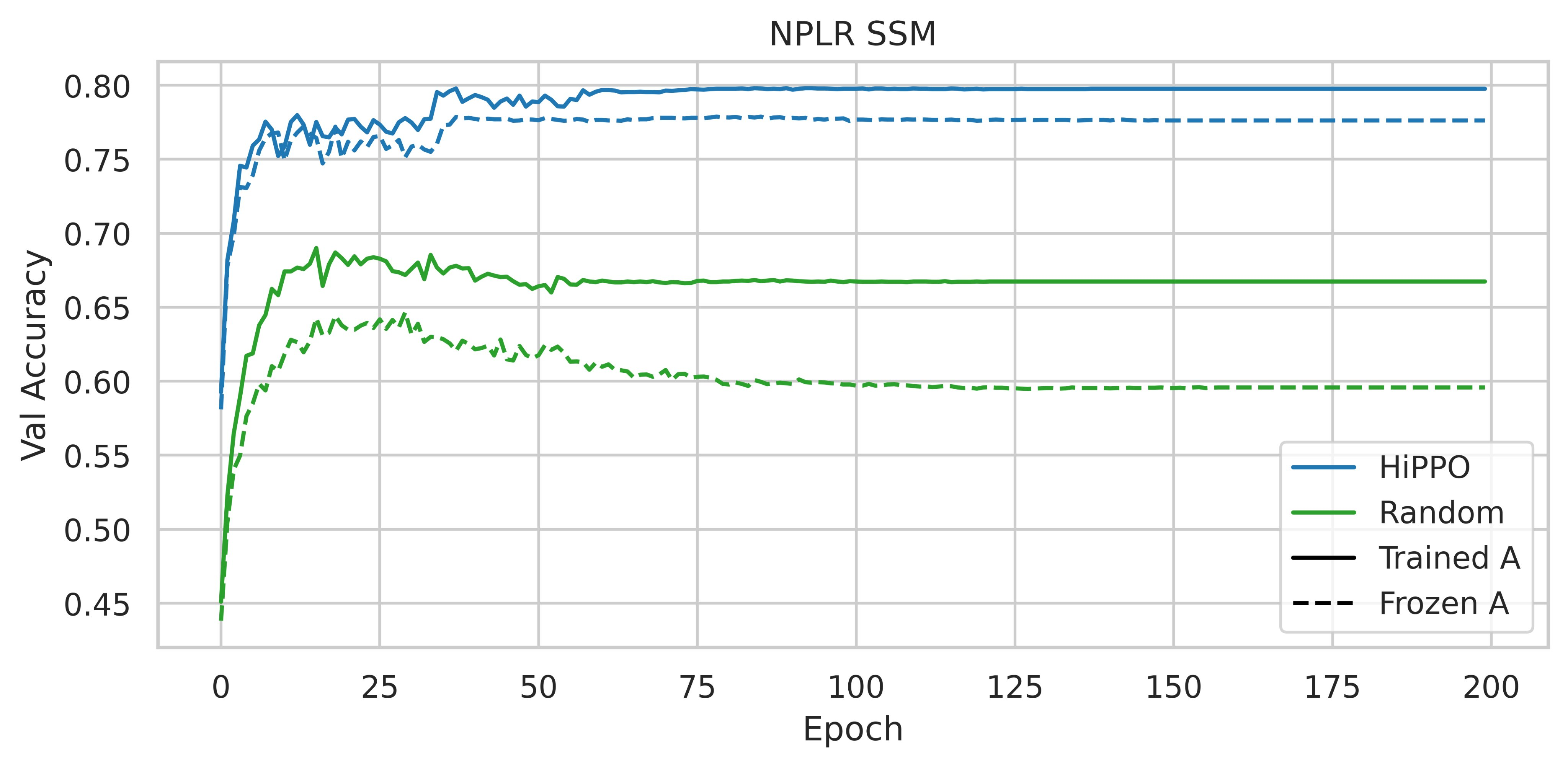
The use of HiPPO is therefore important. Are the performances obtained due to its specific intrinsic qualities, or could any low-rank normal matrix (NPLR for Normal Plus Low-Rank) suffice?

Figure 3: Accuracy on the CIFAR-10 validation split with different initializations and parameterizations, taken from figure 4 of the S4 paper

Initializing an NPLR matrix with HiPPO significantly enhances performance. Thus, according to these experiments, the HiPPO matrix is essential to obtain a high-performance model.

The authors of S4 have further developed their work, which they presented on June 24, 2022 in the paper How to Train Your HiPPO. This is an extremely detailed paper of over 39 pages.

In this paper, the authors focus on a more intuitive interpretation of MSS as a convolutional model where the convolution kernel is a linear combination of particular basis functions, leading to several generalizations and new methods.
For example, they prove that the $\mathbf{A}\backslash mathbf\{A\}$ matrix of S4 produces exponentially scaled Legendre polynomials (LegS). This gives the system a better ability to model long-term dependencies via very smooth kernels.
The authors also derive a new SSM that produces approximations of truncated Fourier functions (FouT). This method generalizes short-time Fourier transforms and local convolutions (i.e. a standard ConvNet). This SSM can also encode state-of-the-art functions to solve classical memory tasks.
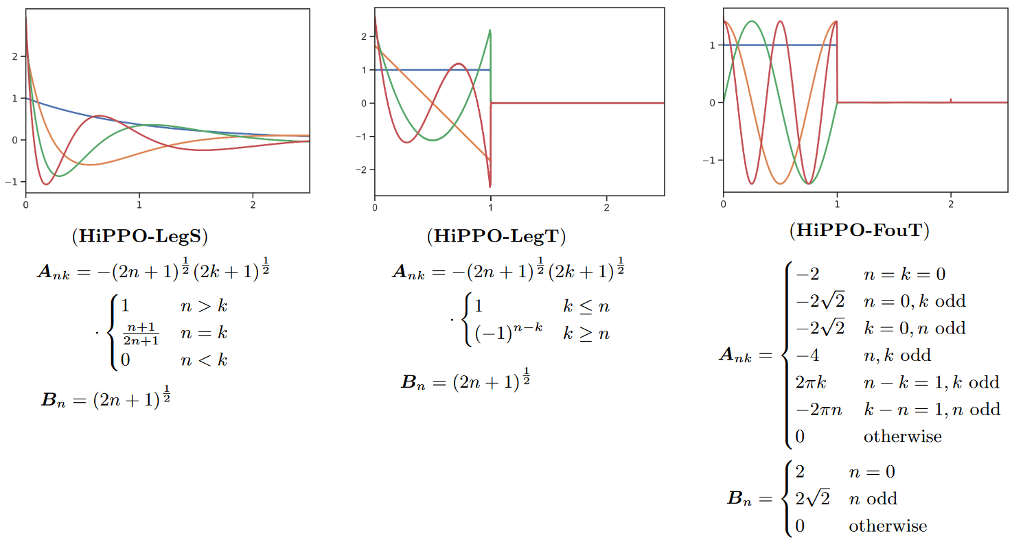
Note that it is mainly HiPPO-FouT that is introduced in this paper, HiPPO-LegS having been introduced in the original HiPPO paper two years earlier. As is HiPPO-LegT (truncated Legendre polynomials).

Figure 4: The different HiPPO variants

The colors represent the first 4 basis functions $K_n(tK\_n(t$) (the convolution kernel) for each of the methods (we invite the reader to look at Table 1 of the paper to see what $K_n(tK\_n(t$) equals for each of the methods).

In addition, the authors also work on the time step $\text{∆}∆$, which independently of a notion of discretization can be interpreted simply as controlling the length of the dependencies or the width of the SSM kernels. The authors also detail how to choose a good value of $\text{∆}∆$ for a given task.

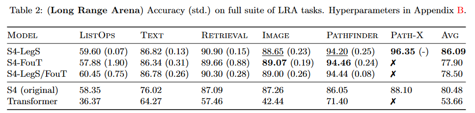
The work carried out improves S4 results by more than 5.5 points on the benchmark LRA by TAY, DEHGHANI et al. (2020):

Figure 5: S4 v2 benchmark results

The model resulting from this paper is generally referred to in the literature as "S4 V2" or "S4 updated", as opposed to the "original S4" or "S4 V1".

DSS: Diagonal State Spaces

On March 27, 2022, Ankit GUPTA introduced Diagonal State Spaces (DSS) in his paper Diagonal State Spaces are as Effective as Structured State Spaces.
It seems that following this paper, he and Albert GU began working together on an updated version of this paper (GU subsequently appearing as co-author in v2 and v3 of the article) and within the framework of S4D (see next section).
The main thing to remember is that this approach is significantly simpler than S4. Indeed, DSS is based on diagonal state matrices (i.e. without the low-rank correction of S4, i.e. without the HiPPO matrix) which, if initialized appropriately, work better than the original S4. The use of a diagonal matrix in place of the HiPPO matrix for $\mathbf{A}\backslash mathbf\{A\}$ has since become standard practice.

Nevertheless, let's dwell on the few complexities/limitations contained in this paper. Listing them will help us understand the contributions of the following methods, which aim to simplify things even further.

1. Discretization
The DSS uses the same system of differential equations as the S4:

However, it uses a different discretization in order to achieve convolutional and recurrent views, namely the zero-order hold (ZOH) discretization, instead of the bilinear discretization, which assumes that the sampled signal is constant between each sampling point.
Below is a table comparing the values of $\mathbf{A}\backslash mathbf\{A\}$, $\mathbf{B}\backslash mathbf\{B\}$ and $\mathbf{C}\backslash mathbf\{C\}$ for each of the two discretizations in the recursive view, as well as the expression of the convolution kernel in the convolutional view:

For the ZOH, after running through the calculations, we end up with $y_k={\sum }_{j=0}^k\bar{C}{\bar{A}}^j\bar{B}\cdot u_{k-j}={\sum }_{j=0}^k{\bar{K}}_j\cdot u_{k-j}y\_k\; =\; \backslash sum\_\{j=0\}^k\; \backslash bar\{C\}\backslash bar\{A\}^j\backslash bar\{B\}\backslash cdot\; u\_\{k-j\}\; =\; \backslash sum\_\{j=0\}^k\; \backslash bar\{K\}\_j\backslash cdot\; u\_\{k-j\}$.

Calculating $yy$ from $uu$ and $\bar{K}\backslash bar\{K\}$ is then done by Fast Fourier Transform (FFT) in $O(Llog(L)O(L~log(L)$) with $LL$ the length of the sequence by simultaneously calculating the multiplication of two polynomials of degrees $L-1L-1$.

2. DSSsoftmax and DSSexp

Short version

GUPTA formulates a proposal to obtain DSS that are as expressive as S4, resulting in the formulation of two different DSS: DSSexp and DSSsoftmax. The information to be retained concerning them can be summarized in the following table:

So we are working here on ℂ and not ℝ.

Long version

GUPTA formulates the following proposition to obtain DSS that are as expressive as S4:

Let $K\in {\mathbb{R}}^{1\times L}K\; \backslash in\; \backslash mathbb\{R\}^\{1\backslash times\; L\}$ be the kernel of length $LL$ of a given state space $(A,B,C(A,\; B,\; C$) and sampling time $\mathrm{\Delta }>0\backslash Delta\; >\; 0$, where $A\in {\mathbb{C}}^{N\times N}A\; \backslash in\; \backslash mathbb\{C\}^\{N\; \backslash times\; N\}$ is diagonalizable on $\mathbb{C}\backslash mathbb\{C\}$ with eigenvalues ${\lambda }_1,\dots ,{\lambda }_N\backslash lambda\_1,\backslash ldots,\backslash lambda\_N$ and $\mathrm{\forall }i\backslash forall\; i$, ${\lambda }_i\mathrm{\ne }0\backslash lambda\_i\; \backslash neq\; 0$ and $e^{L{\lambda }_i\mathrm{\Delta }}\mathrm{\ne }1e^\{L\backslash lambda\_i\backslash Delta\}\; \backslash neq\; 1$. Let $P\in {\mathbb{C}}^{N\times L}{P}_{i,k}={\lambda }_{i}k\mathrm{\Delta }P\; \backslash in\; \backslash mathbb\{C\}^\{N\; \backslash times\; L\}\; P\_\{i,k\}\; =\; \backslash lambda\_i\; k\backslash Delta$ and $\mathrm{\Lambda }\backslash Lambda$ the diagonal matrix with ${\lambda }_1,\dots ,{\lambda }_N\backslash lambda\_1,\backslash ldots,\backslash lambda\_N$. Then there exists $\tilde{w},w\in {\mathbb{C}}^{1\times N}\backslash widetilde\{w\},\; w\; \backslash in\; \backslash mathbb\{C\}^\{1\backslash times\; N\}$ such that :

• (a): $K={\bar{K}}_{\mathrm{\Delta },L}(\mathrm{\Lambda },(1{)}_{1\le i\le N},\tilde{w})=\tilde{w}\cdot {\mathrm{\Lambda }}^{-1}(e^{Lambda\mathrm{\Delta }}-I)\cdot \text{elementwise-exp}(P)K\backslash \; =\backslash \; \backslash bar\{K\}\_\{\backslash Delta,\; L\}(\backslash Lambda,\backslash \; (1)\_\{1\; \backslash leq\; i\; \backslash leq\; N\},\backslash \; \backslash widetilde\{w\})\backslash \; =\backslash \; \backslash widetilde\{w\}\; \backslash cdot\; \backslash Lambda^\{-1\}\; (e^\{Lambda\backslash Delta\}\; -\; I)\; \backslash cdot\; \backslash text\{elementwise-exp\}(P)$
• (b): $K={\bar{K}}_{\mathrm{\Delta },L}(\mathrm{\Lambda },((e^{Lambd{a}_i\mathrm{\Delta }}-1{)}^{-1}{)}_{1\le i\le N},w)=w\cdot {\mathrm{\Lambda }}^{-1}\cdot \text{row-softmax}(P)K\backslash \; \backslash \; =\backslash \; \backslash bar\{K\}\_\{\backslash Delta,\; L\}(\backslash Lambda,\backslash \; ((e^\{Lambda\_i\backslash Delta\}\; -\; 1)^\{-1\})\_\{1\backslash leq\; i\; \backslash leq\; N\},\backslash \; w)\backslash \; =\backslash \; \backslash \; w\; \backslash cdot\; \backslash Lambda^\{-1\}\; \backslash cdot\; \backslash text\{row-softmax\}(P)$

(a) suggests that we can parameterize the state spaces via $\mathrm{\Lambda },\tilde{w}\in {\mathbb{C}}^N\backslash Lambda,\; \backslash widetilde\{w\}\; \backslash in\; \backslash mathbb\{C\}^N$ and compute the kernel as shown. Unfortunately, in practice, the real part of the elements of $\mathrm{\Lambda }\Lambda$ may become positive during learning, making it unstable for long inputs. To solve this problem, the authors propose two methods: DSSexp and DSSsoftmax.

2.1 Convolutional view
In DSSexp, the real parts of $\mathrm{\Lambda }\Lambda$ must be negative. We then have $\mathrm{\Lambda }=-\text{elementwise-exp}({\mathrm{\Lambda }}_{\mathrm{r}\mathrm{e}})+i\cdot {\mathrm{\Lambda }}_{\mathrm{i}\mathrm{m}}\backslash Lambda\; =\; -\; \backslash text\{elementwise-exp\}(\backslash Lambda\_\backslash mathrm\{re\})\; +\; i\backslash cdot\; \backslash Lambda\_\backslash mathrm\{im\}$ and $\mathrm{\Delta }=\mathrm{e}\mathrm{x}\mathrm{p}({\mathrm{\Delta }}_{\log })\in {\mathbb{R}}_{>0}\backslash Delta\; =\; \backslash mathrm\{exp\}(\backslash Delta\_\{\backslash log\})\; \backslash in\; \backslash mathbb\{R\}\_\{>\; 0\}$. $KK$ is then calculated as in the formula given in part (a) of the proposal.
In DSSsoftmax, each line of $\mathrm{\Lambda }\Lambda$ is normalized by the sum of these elements. We have $\mathrm{\Lambda }={\mathrm{\Lambda }}_{\mathrm{r}\mathrm{e}}+i\cdot {\mathrm{\Lambda }}_{\mathrm{i}\mathrm{m}}\backslash Lambda\; =\; \backslash Lambda\_\backslash mathrm\{re\}\; +\; i\backslash cdot\; \backslash Lambda\_\backslash mathrm\{im\}$ and $\mathrm{\Delta }=\mathrm{e}\mathrm{x}\mathrm{p}({\mathrm{\Delta }}_{\log })\in {\mathbb{R}}_{>0}\backslash Delta\; =\; \backslash mathrm\{exp\}(\backslash Delta\_\{\backslash log\})\; \backslash in\; \backslash mathbb\{R\}\_\{>\; 0\}$. $KK$is then calculated as in the formula indicated in part (b) of the proposition.
Note that softmax on $\mathbb{C}\backslash mathbb\{C\}$ is not necessarily defined during sofmax $(0,i\pi )(0,\; i\; \backslash pi)$, the authors using a corrected version of softmax to prevent this problem (see Appendix A.2. of the paper).

2.2 Recurrence view
In DSSexp, using the recurrence formula in the table above, we obtain $\bar{A}=\mathrm{d}\mathrm{i}\mathrm{a}\mathrm{g}(e^{lambd{a}_1\mathrm{\Delta }},\dots ,e^{lambd{a}_N\mathrm{\Delta }})\backslash bar\{A\}\; =\; \backslash mathrm\{diag\}(e^\{lambda\_1\backslash Delta\},\; \backslash ldots,\; e^\{lambda\_N\backslash Delta\})$ and $\bar{B}={({\lambda }_i^{-1}(e^{lambd{a}_i\mathrm{\Delta }}-1))}_{1\le i\le N}\backslash bar\{B\}\; =\; \backslash left(\backslash lambda\_i^\{-1\}\; (e^\{lambda\_i\backslash Delta\}\; -\; 1)\; \backslash right)\_\{1\backslash leq\; i\; \backslash leq\; N\}$, where in both equalities, ${\lambda }_i\backslash lambda\_i$ is Lambda's ith eigenvalue.
Since $\bar{A}\backslash bar\{A\}$ is diagonal, we can calculate $x_{k}x\_k$ independently as follows: $x_{i,k}=e^{{\lambda }_i\mathrm{\Delta }}{x}_{i,k-1}+{\lambda }_i^{-1}(e^{{\lambda }_i\mathrm{\Delta }}-1)u_{k}x\_\{i,k\}\; =\; e^\{\backslash lambda\_i\backslash Delta\}\; x\_\{i,k-1\}\; +\; \backslash lambda\_i^\{-1\}\; (e^\{\backslash lambda\_i\backslash Delta\}\; -\; 1)u\_k$.
It is then possible to deduce that, if ${\lambda }_i\mathrm{\mid }\mathrm{\Delta }\approx 0\backslash lambda\_i|\backslash Delta\; \backslash approx\; 0$, we have $x_{i,k}\approx x_{i,k-1}x\_\{i,k\}\; \backslash approx\; x\_\{i,k-1\}$ allowing us to copy the story over many time steps. On the other hand, if $\mathrm{R}\mathrm{e}({\lambda }_i)\mathrm{\Delta }\ll 0\backslash mathrm\{Re\}(\backslash lambda\_i)\backslash Delta\; \backslash ll\; 0$, then ${}_{i,k}\approx -{\lambda }_i^{-1}{u}_k\_\{i,k\}\; \backslash approx\; -\backslash lambda\_i^\{-1\}u\_k$ and information from previous time steps is forgotten, similar to a "forget" gate in LSTMs.

In DSSsoftmax, using the recurrence formula in the table above, we obtain: $\bar{A}=\mathrm{d}\mathrm{i}\mathrm{a}\mathrm{g}(e^{ambd{a}_1\mathrm{\Delta }},\dots ,e^{ambd{a}_N\mathrm{\Delta }})\backslash bar\{A\}\; =\; \backslash mathrm\{diag\}(e^\{ambda\_1\backslash Delta\},\; \backslash ldots,\; e^\{ambda\_N\backslash Delta\})$ and $barB={\left(\frac{e^{ambd{a}_i\mathrm{\Delta }}-1}{{\lambda }_i(e^{ambd{a}_i\mathrm{\Delta }L}-1)}\right)}_{1\le i\le N}bar\{B\}\; =\; \backslash left(\; \{e^\{ambda\_i\backslash Delta\}\; -\; 1\; \backslash over\; \backslash lambda\_i\; (e^\{ambda\_i\backslash Delta\; L\}\; -\; 1)\}\; \backslash right)\_\{1\backslash leq\; i\; \backslash leq\; N\}$.
Hence $x_{i,k}=e^{{\lambda }_i\mathrm{\Delta }}{x}_{i,k-1}+\frac{u_k(e^{{\lambda }_i\mathrm{\Delta }}-1)}{{\lambda }_i(e^{{\lambda }_i\mathrm{\Delta }L}-1)}x\_\{i,k\}\; =\; e^\{\backslash lambda\_i\backslash Delta\}\; x\_\{i,k-1\}\; +\; \{u\_k(e^\{\backslash lambda\_i\backslash Delta\}\; -\; 1)\; \backslash over\; \backslash lambda\_i\; (e^\{\backslash lambda\_i\backslash Delta\; L\}\; -\; 1)\}$.
Note that $e^{{\lambda }_i\mathrm{\Delta }}e^\{\backslash lambda\_i\backslash Delta\}$ can be unstable. We must then calculate two different cases depending on the sign of $\mathrm{R}\mathrm{e}(\lambda )\backslash mathrm\{Re\}(\backslash lambda)$ by introducing an intermediate state ${\tilde{x}}_k\backslash widetilde\{x\}\_\{k\}$.
• If $\mathrm{R}\mathrm{e}(\lambda )\le 0\backslash mathrm\{Re\}(\backslash lambda)\; \backslash leq\; 0$: ${\tilde{x}}_k=e^{\lambda \mathrm{\Delta }}\cdot {\tilde{x}}_{k-1}+u_k,x_k={\tilde{x}}_k\cdot \frac{(e^{\lambda \mathrm{\Delta }}-1)}{\lambda (e^{\lambda \mathrm{\Delta }L}-1)}\backslash widetilde\{x\}\_\{k\}\; =\; e^\{\backslash lambda\backslash Delta\}\backslash cdot\; \backslash widetilde\{x\}\_\{k-1\}\; +\; u\_k\; \backslash \; \backslash \; \backslash \; ,\backslash \; \backslash \; \backslash \; x\_k\; =\; \backslash widetilde\{x\}\_k\; \backslash cdot\; \{(e^\{\backslash lambda\backslash Delta\}\; -\; 1)\; \backslash over\; \backslash lambda\; (e^\{\backslash lambda\backslash Delta\; L\}\; -\; 1)\; \}$.

And in particular if $\mathrm{R}\mathrm{e}(\lambda )\ll 0\backslash mathrm\{Re\}(\backslash lambda)\; \backslash ll\; 0$ then ${\tilde{x}}_k\approx u_k\backslash widetilde\{x\}\_k\; \backslash approx\; u\_k$ and $x_k\approx u_k\mathrm{/}\lambda x\_k\; \backslash approx\; u\_k\; /\; \backslash lambda$, resulting in a focus on local information (previous steps are ignored).

• If $\mathrm{R}\mathrm{e}(\lambda )>0\backslash mathrm\{Re\}(\backslash lambda)\; >\; 0$: ${\tilde{x}}_k={\tilde{x}}_{k-1}+e^{-k\lambda \mathrm{\Delta }}\cdot u_k,x_k={\tilde{x}}_k\cdot \frac{e^{lambda\mathrm{\Delta }(k-(L-1))}}{\lambda }\cdot \frac{e^{-\lambda \mathrm{\Delta }}-1}{e^{-\lambda \mathrm{\Delta }L}-1}\backslash widetilde\{x\}\_\{k\}\; =\; \backslash widetilde\{x\}\_\{k-1\}\; +\; e^\{-k\backslash lambda\backslash Delta\}\; \backslash cdot\; u\_k\; \backslash \; \backslash \; \backslash \; \backslash \; ,\backslash \; \backslash \; \backslash \; \backslash \; x\_k\; =\; \backslash widetilde\{x\}\_k\; \backslash cdot\; \{e^\{lambda\backslash Delta\; (k-(L-1))\}\; \backslash over\; \backslash lambda\}\backslash cdot\; \{e^\{-\backslash lambda\backslash Delta\}-1\; \backslash over\; e^\{-\backslash lambda\backslash Delta\; L\}\; -\; 1\; \}$

Similarly if $\mathrm{R}\mathrm{e}(\lambda )\gg 0\backslash mathrm\{Re\}(\backslash lambda)\; \backslash gg\; 0$ then ${\tilde{x}}_0\approx u_0\backslash widetilde\{x\}\_0\; \backslash approx\; u\_0$ and ${\tilde{x}}_k\approx {\tilde{x}}_{k-1}\approx u_0\backslash widetilde\{x\}\_k\; \backslash approx\; \backslash widetilde\{x\}\_\{k-1\}\; \backslash approx\; u\_0$, and $x_{L-1}\approx u_0\mathrm{/}\lambda x\_\{L-1\}\; \backslash approx\; u\_0\; /\; \backslash lambda$, the model can capture information at very long distances. In practice, the authors of S4D indicate that $\mathrm{R}\mathrm{e}(\lambda )\gg 0\backslash mathrm\{Re\}(\backslash lambda)\; \backslash gg\; 0$ doesn't work if $LL$ is very large (explosion when $t\to \mathrm{\infty }t\; \backslash rightarrow\; \backslash infty$ in $K(t)=C\exp (A^{⊺})\mathrm{.}B)K(t)\; =\; C\; \backslash exp(A^\backslash intercal).B)$.

3. Initialization
The real and imaginary parts of $ww$ are initialized from $\mathcal{N}(0,1)\backslash mathcal\{N\}(0,1)$, the elements of ${\mathrm{\Delta }}_{\log }\backslash Delta\_\{\backslash log\}$ from $\exp (\mathcal{U}(log(0.001),log(0.1)))\backslash exp(\backslash mathcal\{U\}~(log(0.001),\; log(0.1)))$, and $\mathrm{\Delta }\backslash Delta$ via the eigenvalues of the HiPPO matrix. The authors wonder whether it might not be possible to find a simpler initialization for $\mathrm{\Delta }\backslash Delta$. They note, however, that randomization leads to poorer results.

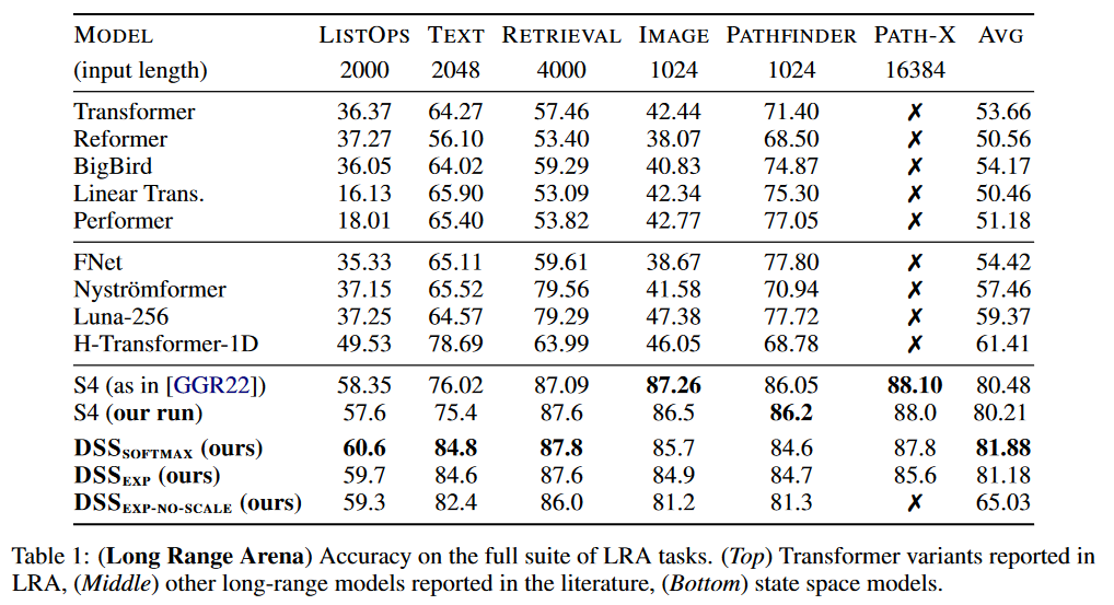
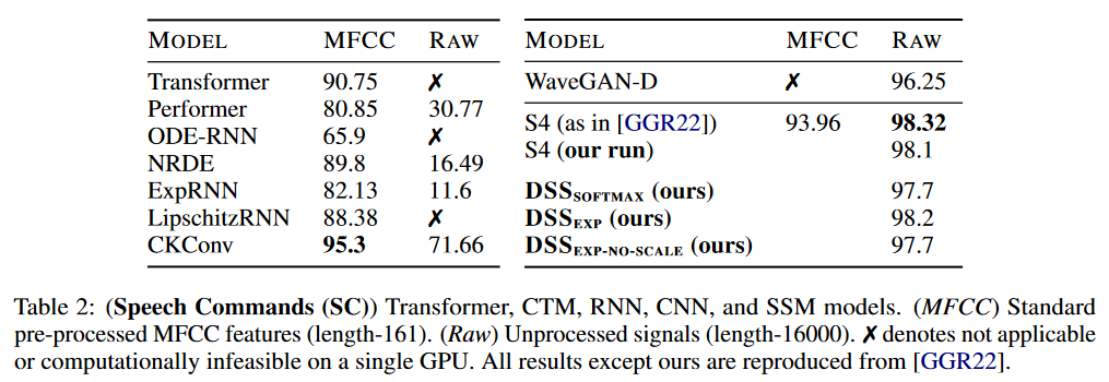
Regarding the results, DSS has been tested on LRA and Speech Commands by WARDEN (2018):

Figure 6: DSS results on LRA

The DSS (in softmax or exp versions) achieves better average results than the original S4 for this benchmark. DSSsoftmax seems to perform slightly better than DSSexp. Another interesting aspect of this paper is that it is the first to reproduce the S4 results, thus confirming that SSMs pass this benchmark.

Figure 7: DSS results on Speech Commands

On Speech Commands, the S4 maintains its advantage over DSS.

To dig deeper
The official implementation is available on GitHub.
This paper was the subject of a spotlight talk at NeurIPS 2022.

S4D: the diagonal S4

On June 23, 2022, GU, GUPTA et al. introduced S4D in their paper On the Parameterization and Initialization of Diagonal State Space Models.
Initialization of the DSS state matrix $\mathbf{A}\backslash mathbf\{A\}$ relies on a particular approximation of the S4 HiPPO matrix. While the S4 matrix has a mathematical interpretation for dealing with long-range dependencies, the effectiveness of the diagonal approximation remains theoretically unexplained.
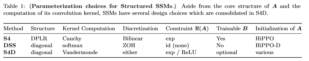
With S4D, the authors introduce a diagonal SSM combining the best of S4 computation and parameterization and DSS initialization. The result is a very simple, theoretically sound and empirically effective method.

A comparison of the three methods is given in Table 1 of the paper:

Figure 8: Comparison of S4, DSS and S4D

S4D can use either the bilinear discretization of S4 or the ZOH discretization of DSS.

In S4D, the discretized convolution kernel of the equation $y=u\ast \bar{\mathbf{K}}y\; =\; u\; \backslash ast\; \backslash mathbf\{\backslash overline\{K\}\}$ is calculated as follows:
${\bar{\mathbf{K}}}_{\mathrm{\ell }}={\sum }_{n=0}^{N-1}{\mathbf{C}}_n{\bar{\mathbf{A}}}_n^{\mathrm{\ell }}{\bar{\mathbf{B}}}_n⟹\bar{\mathbf{K}}=({\bar{\mathbf{B}}}^{\mathrm{\top }}\circ \mathbf{C})\cdot {\mathcal{V}}_L(\bar{\mathbf{A}})\backslash mathbf\{\backslash overline\{K\}\}\_\backslash ell\; =\; \backslash sum\_\{n\; =\; 0\}^\{N-1\}\; \backslash mathbf\{C\}\_n\; \backslash mathbf\{\backslash overline\{A\}\}\_n^\backslash ell\; \backslash mathbf\{\backslash overline\{B\}\}\_n\; \backslash implies\; \backslash mathbf\{\backslash overline\{K\}\}\; =\; (\backslash mathbf\{\backslash overline\{B\}\}^\backslash top\; \backslash circ\; \backslash mathbf\{C\})\; \backslash cdot\; \backslash mathcal\{V\}\_L(\backslash mathbf\{\backslash overline\{A\}\})$
where :
• $\circ \backslash circ$ represents the Hadamard matrix product,
• $\cdot \backslash cdot$ a classic matrix product,
• ${\mathcal{V}}_L\backslash mathcal\{V\}\_L$ is the Vandermonde matrix i.e.: .

In other words, for any $ii$ and $jj$, the coefficient in row $ii$ and column $jj$ is ${\displaystyle V_{i,j}={{\alpha }_i}^{j-1}}\backslash displaystyle\; V\_\{i,j\}=\{\backslash alpha\; \_\{i\}\}^\{j-1\}$.

Finally, in S4D,

All calculable in $O(N+L)O(N+L)$ operations and space.

The parametrization of the various matrices is as follows:

• $\mathbf{A}=-\exp (\mathrm{\Re }(\mathbf{A}))+i\cdot \mathrm{\Im }(\mathbf{A})\backslash mathbf\{A\}\; =\; -\backslash exp(\backslash Re(\backslash mathbf\{A\}))\; +\; i\; \backslash cdot\; \backslash Im(\backslash mathbf\{A\})$.
  The authors point out that the exponential can be replaced by any positive function.
• $\mathbf{B}=1\backslash mathbf\{B\}\; =\; 1$ then is trained
• $\mathbf{C}\backslash mathbf\{C\}$ random with a standard deviation of 1 then trained.

Note that S4 takes real numbers into account, whereas S4D takes complex numbers into account by parameterizing with a state size of $N\mathrm{/}2N/2$ and implicitly adding conjugate pairs to the parameters. We then have the equivalent of $NN$ real parameters ensuring that the output is real.

Concerning initialization, the authors introduce two:

• S4D-Inv is an approximation of S4-LegS: ${\mathbf{A}}_n=-\frac{1}{2}+i\frac{N}{\pi }(\frac{N}{2n+1}-1)\backslash quad\; \backslash mathbf\{A\}\_n\; =\; -\backslash frac\{1\}\{2\}\; +\; i\; \backslash frac\{N\}\{\backslash pi\}\; \backslash left(\; \backslash frac\{N\}\{2n+1\}-1\; \backslash right)$
• S4D-Lin which is an approximation of S4-FouT: ${\mathbf{A}}_n=-\frac{1}{2}\mathbf{1}+i\pi n\backslash quad\; \backslash mathbf\{A\}\_n\; =\; -\backslash frac\{1\}\{2\}\backslash mathbf\{1\}\; +\; i\; \backslash pi\; n$.

We invite the reader to consult part 4 of the paper for more details on these equations.
From an interpretability point of view, the real part of ${\mathbf{A}}_n\backslash mathbf\{A\}\_n$ controls the rate of weight decay. The imaginary part of ${\mathbf{A}}_n\backslash mathbf\{A\}\_n$ controls the oscillation frequencies of the basis function $K_n(t)=e^{t\mathbf{A}}\mathbf{B}K\_n(t)\; =\; e^\{t\backslash mathbf\{A\}\}\backslash mathbf\{B\}$.

Finally, the authors put forward a few results:

1. Calculating the model with a softmax instead of Vandermonde doesn't make much difference
2. Training B always gives better results.
3. There are no significant differences between the two possible discretizations.
4. Restricting the real part of A leads to better results (although not significantly).
5. All the modifications tested for initialization degraded the results. Namely, applying a coefficient to the imaginary part or using a random imaginary part / using a random real part / using an imaginary part and a random real part.

As this method is much easier to implement than the others (Vandermade requires just two lines of code), S4D has replaced S4 in common usage (in fact, in table 6 of the Mamba paper, for example, the authors use the term S4 to designate S4D).

To dig deeper
The official implementation is available on GitHub.
On December 1, 2022, GUPTA et al. present a sequel to DSS with Simplifying and Understanding State Space Models with Diagonal Linear RNNs which introduces DLR. They get rid of the discretization step and propose a model based on diagonal linear RNNs (DLR) that can operate on around 1 million positions (unlike classic RNNs). The code for this model is available on GitHub.

GSS: Gated State Space

Five days after S4D, on June 27, 2022, MEHTA, GUPTA et al. introduce GSS in their paper Long Range Language Modeling via Gated State Spaces.
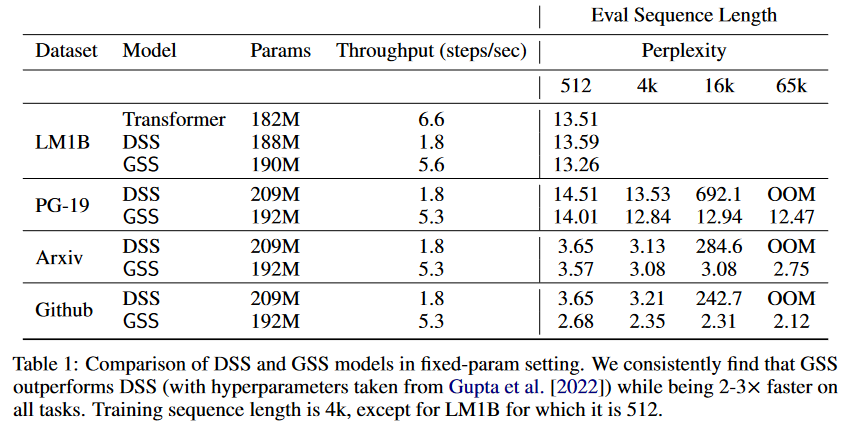
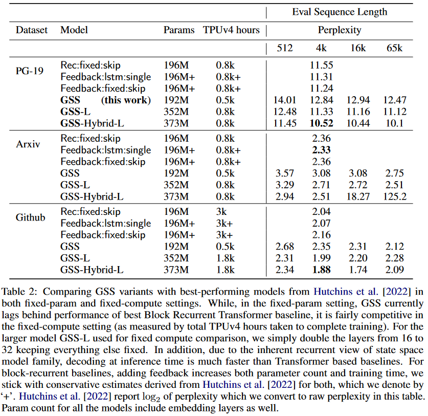
In this work, they focus on modeling autoregressive sequences (where previous work on GSS focused particularly on sequence classification tasks) from English books, Github source code and ArXiv mathematical articles. They show that their layer called Gated State Space (GSS) trains significantly faster than DSS (2 to 3 times faster). They also show that exploiting self-attention to model local dependencies further improves GSS performance.

Figure 9: Comparison of DSS vs GSS. Models are trained on sequences of 4K length and then evaluated on sequences of up to 65K tokens.

Based on the observation that SSMs (S4/DSS) train more slowly than expected on TPU, the authors modified the architecture to reduce the dimensionality of specific operations that proved to be bottlenecks. These modifications are inspired by well-supported empirical observation regarding the efficiency of gating units (Language Modeling with Gated Convolutional Networks by DAUPHIN et al. (2016), GLU Variants Improve Transformer by SHAZEER (2020), etc.). More specifically, the authors draw inspiration from the paper Transformer Quality in Linear Time by HUA et al. (2022). The latter showed that with their FLASH model, replacing the feed-forward layer in the Transformer with gating units enables the use of lower unit-peak attention with minimal quality loss. They call this component the Gated Attention Unit (GAU).

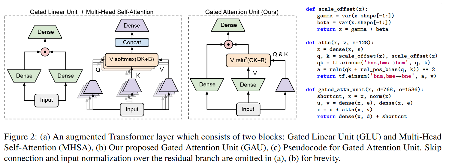Figure 10: The Gated Attention Unit. This is not exactly the same figure as the one on the paper: I've made a horizontal translation so that the input is at the bottom and not at the top, to facilitate the parallel with the Mega figure visible below.

The authors of GSS have therefore extended the use of gating units to SSMs, and observe a reduction in dimensionality when performing FFT operations.

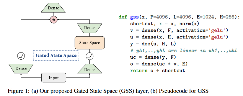Figure 11: Adaptation of GAU to SSM.

Note that unlike HUA et al. the authors do not observe much advantage in using RELU² or Swish activations instead of GELU hence its retention.
In addition, DSS uses a time step $\text{∆}∆$ fixed at 1 (the authors observing that this reduces the computational time required to create the kernels and simplifies their calculation).
A particularly interesting point is that, in contrast to the observations made in S4 and DSS, the model's performance on language modeling tasks was found to be much less sensitive to initialization allowing then to train the model successfully by initializing the state space variables randomly. This is a very important result, as it shows that neither the HiPPO matrix (S4) nor the HiPPO initialization (DSS) are necessary.

As for the GSS-Transformer hybrid, it simply consists of sparingly interspersing traditional Transformer blocks with GSS layers. The hybrid model achieves lower perplexity than the pure SSM model:

Figure 12: Performance of the GSS-Transformer hybrid model.

To dig deeper
The official implementation is available on GitHub.

Mega

On September 21, 2022, MA, ZHOU et al. published the Mega: Moving Average Equipped Gated Attention.
The Mega is a transformer with a single-headed attention mechanism, using the GAU gating system, and is equipped with a damped exponential moving average (EMA) to incorporate positional inductive bias.

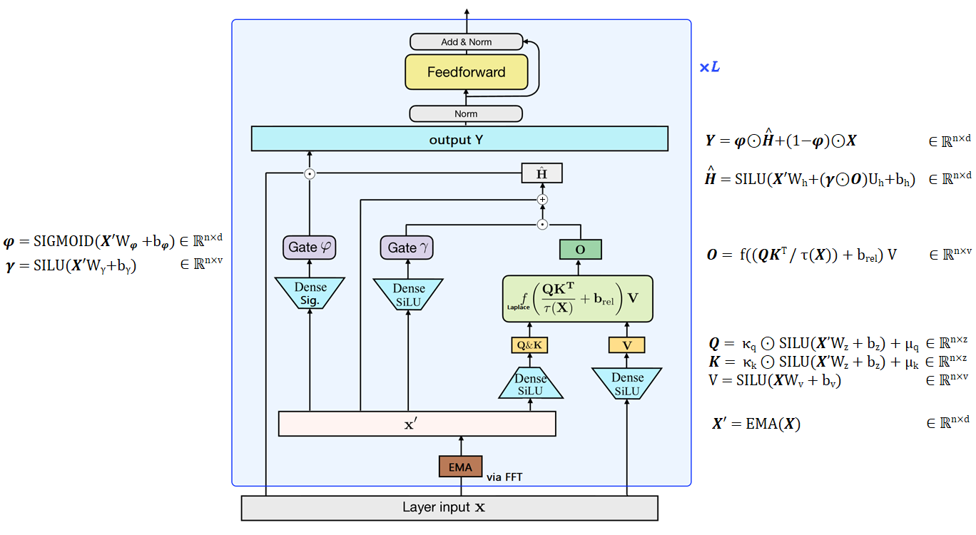Figure 13: Overview of the Mega, figure designed from my understanding of the paper. The authors replace the RELU² of the GAU with a Laplace function which is more stable (cf. figure 4 in the paper).

The authors also propose a variant, Mega-chunk, which effectively divides the entire sequence into several fixed-length chunks. Here, they take up the principle already present and explained in the FLASH model (see figure 4 of the paper on this model). This offers linear complexity in terms of time and space with minimal loss of quality.

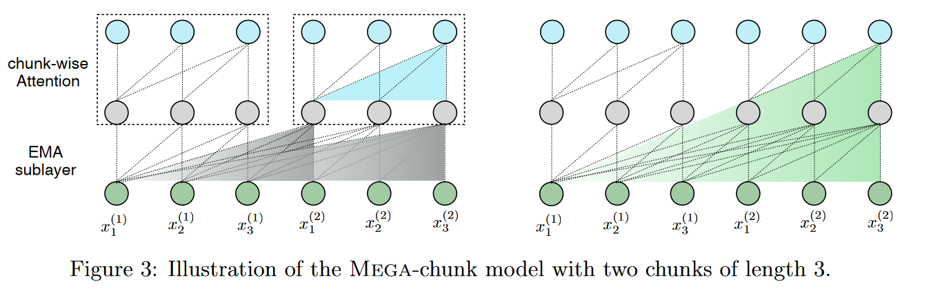Figure 14: The Mega chunk

This offers linear complexity, simply applying attention locally to each fixed-length chunk.
More precisely, we divide the sequences of queries, keys and values into chunks of length $cc$. For example, $\mathbf{Q}={\mathbf{Q}}_1,\mathrm{.}\mathrm{.}\mathrm{.}{\mathbf{Q}}_k\backslash mathbf\{Q\}\; =\; \{\backslash mathbf\{Q\}\_1,\; ...\; \backslash mathbf\{Q\}\_k\}$, where $k=-\frac{n}{c}k\; =\; -\backslash frac\{n\}\{c\}$ is the number of chunks. The attention operation is applied individually to each block, giving a linear complexity $\mathcal{O}(k{c}^2)=\mathcal{O}(nc)\backslash mathcal\{O\}(kc^2)\; =\; \backslash mathcal\{O\}(nc)$ with respect to $nn$.
Nevertheless, this method suffers from a critical limitation, namely the loss of contextual information from other blocks. But the EMA sublayer mitigates this problem by capturing local contextual information in the vicinity of each token whose results are used as inputs to the attention sublayer. In this way, the effective context exploited by attention at block level can extend beyond the block boundary.

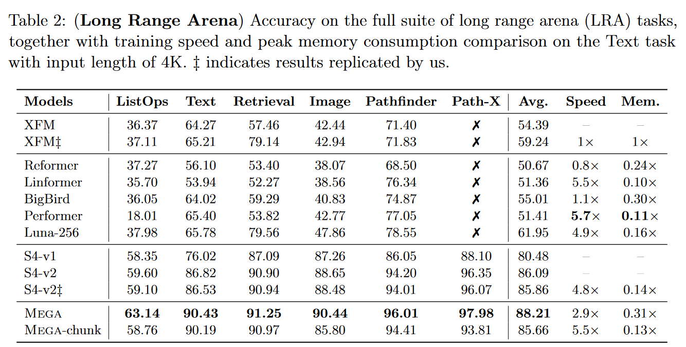
Mega is extremely competitive, as it becomes the best model on the LRA:

Figure 15: Mega's results on the LRA benchmark

So what's a transformer doing in a blog post about SSM? Let's look at damped EMA to understand the link between Mega and S4D.

• Reminder on "classic" EMA:
The equation of a "classical" EMA is ${𝐲}_t=\text{𝜶}\odot {𝐱}_t+(1-\text{𝜶})\odot {𝐲}_{t-1}𝐲\_t\; =\; 𝜶\; \odot \; 𝐱\_t\; +\; (1-𝜶)\; \odot \; 𝐲\_\{t-1\}$ with $\text{𝜶}𝜶$ in $[0,1{]}^d[0,1]^d$ the EMA coefficient representing the degree of weighting decrease and ⊙ the Hadamard matrix product.
A higher 𝜶 discounts older observations more quickly.
We therefore impose an inductive bias here: the weight of the dependency between two tokens decreases exponentially over time with an input-agnostic 𝜶 factor. This property favors local dependencies and limits long-term dependencies.
The EMA calculation can be represented as n individual convolutions that can be efficiently calculated by FFT.

• EMA used in the Mega:
The Mega uses a multidimensional "damped" EMA. That is, in the "damped" EMA equation, ${𝐲}_t=\text{𝜶}\odot {𝐱}_t+(1-\text{𝜶}\odot \text{𝜹})\odot {𝐲}_{t-1}𝐲\_t\; =\; 𝜶\; \odot \; 𝐱\_t\; +\; (1-𝜶\; \odot \; 𝜹)\; \odot \; 𝐲\_\{t-1\}$ where a parameter $\text{𝜹}𝜹$ in $[0,1{]}^d[0,\; 1]^d$ is introduced which represents the damping factor, $xx$ is extended to $hh$ dimensions via an expansion matrix $\text{𝜷}𝜷$ in $R^{d\times h}R^\{d\; \backslash times\; h\}$.
The equation then becomes ${𝐲}_{t,j}={\text{𝜼}}_j^{⊺}{𝐡}_t^{(j)}𝐲\_\{t,\; j\}\; =\; 𝜼\_j^\{\backslash intercal\}\; 𝐡\_t^\{(j)\}$ with ${𝐡}_t^{(j)}={\text{𝜶}}_j\odot {𝐮}_t^{(j)}+(1-{\text{𝜶}}_j\odot {\text{𝜹}}_j)\odot {𝐡}_{t-1}^{(j)}𝐡\_t^\{(j)\}\; =\; 𝜶\_j\; \odot \; 𝐮\_t^\{(j)\}+\; (1-𝜶\_j\; \odot \; 𝜹\_j)\; \odot \; 𝐡\_\{t-1\}^\{(j)\}$ and $\text{𝜼}\in R^{d\times h}𝜼\; \backslash in\; R^\{d\; \backslash times\; h\}$ is the projection matrix that returns the $hh$-dimensional hidden state to the 1-dimensional output ${𝐲}_{t,j}\in \mathbb{R}𝐲\_\{t,\; j\}\; \backslash in\; \backslash mathbb\{R\}$.

Proof that multidimensional "damped" EMA can be computed as a convolution and therefore by FTT (by setting $d=1d\; =\; 1$ for $\text{𝜶}𝜶$ and $\text{𝜹}𝜹$) :

We have ${𝐲}_t={\text{𝜼}}^{⊺}{𝐡}_t𝐲\_t\; =\; 𝜼^\{\backslash intercal\}\; 𝐡\_t$ with ${𝐡}_t={\text{𝜶}}_j\odot {𝐮}_t+(1-\text{𝜶}\odot \text{𝜹})\odot {𝐡}_{t-1}𝐡\_t\; =\; 𝜶\_j\; \odot \; 𝐮\_t\; +\; (1-𝜶\; \odot \; 𝜹)\; \odot \; 𝐡\_\{t-1\}$. Let's note $\varphi =1-\text{𝜶}\odot \text{𝜹}\varphi \; =\; 1-𝜶\; \odot \; 𝜹$.
Then: ${𝐡}_t=\text{𝜶}\odot {𝐮}_t+(1-\text{𝜶}\odot \text{𝜹})\odot {𝐡}_{t-1}=\text{𝜶}\odot \text{𝜷}{𝐱}_t+\varphi \odot {𝐡}_{t-1}𝐡\_t\; =\; 𝜶\; \odot \; 𝐮\_t\; +\; (1-𝜶\; \odot \; 𝜹)\; \odot \; 𝐡\_\{t-1\}\; =\; 𝜶\; \odot \; 𝜷\; 𝐱\_t\; +\; \varphi \; \odot \; 𝐡\_\{t-1\}$
    and ${𝐲}_t={\text{𝜼}}^{⊺}{𝐡}_t={\text{𝜼}}^{⊺}(\text{𝜶}\odot \text{𝜷}{𝐱}_t+\varphi \odot {𝐡}_{t-1})𝐲\_t\; =\; 𝜼^\{\backslash intercal\}\; 𝐡\_t\; =\; 𝜼^\{\backslash intercal\}\; (𝜶\; \odot \; 𝜷\; 𝐱\_t\; +\; \varphi \; \odot \; 𝐡\_\{t-1\})$
Then, unrolling the two equations above, we explicitly obtain:
Step 0: ${𝐡}_1=\text{𝜶}\odot \text{𝜷}{𝐱}_1+\varphi \odot {𝐡}_0𝐡\_1\; =\; 𝜶\; \odot \; 𝜷𝐱\_1\; +\; \varphi \; \odot \; 𝐡\_0$
Step 1: ${𝐡}_2=\text{𝜶}\odot \text{𝜷}{𝐱}_2+\varphi \odot {𝐡}_1𝐡\_2\; =\; 𝜶\; \odot \; 𝜷𝐱\_2\; +\; \varphi \; \odot \; 𝐡\_1$ $=\text{𝜶}\odot \text{𝜷}{𝐱}_2+\varphi \odot (\varphi \odot {𝐡}_0+\text{𝜶}\odot \text{𝜷}{𝐱}_1)=\text{𝜶}\odot \text{𝜷}{𝐱}_2+{\varphi }^2\odot {𝐡}_0+\varphi \odot \text{𝜶}\odot \text{𝜷}{𝐱}_1=\; 𝜶\; \odot \; 𝜷\; 𝐱\_2\; +\; \varphi \; \odot \; (\varphi \; \odot \; 𝐡\_0\; +\; 𝜶\; \odot \; 𝜷\; 𝐱\_1)\; =\; 𝜶\; \odot \; 𝜷\; 𝐱\_2\; +\; \varphi ^2\; \odot \; 𝐡\_0\; +\; \varphi \; \odot \; 𝜶\; \odot \; 𝜷\; 𝐱\_1$
...

And likewise:
Step 0: ${𝐲}_1={\text{𝜼}}^{⊺}\text{𝜶}\odot \text{𝜷}{𝐱}_1+\varphi \odot 𝐡0)={\text{𝜼}}^{⊺}\text{𝜶}\odot \text{𝜷}{𝐱}_1+{\text{𝜼}}^{⊺}\varphi \odot {𝐡}_0𝐲\_1\; =\; 𝜼^\{\backslash intercal\}\; 𝜶\; \odot \; 𝜷\; 𝐱\_1\; +\; \varphi \; \odot 𝐡0)\; =\; 𝜼^\{\backslash intercal\}\; 𝜶\; \odot \; 𝜷\; 𝐱\_1\; +\; 𝜼^\{\backslash intercal\}\; \varphi \; \odot \; 𝐡\_0$
Step 1: ${𝐲}_2={\text{𝜼}}^{⊺}\text{𝜶}\odot \text{𝜷}{𝐱}_2+{\text{𝜼}}^{⊺}\varphi \odot {𝐡}_1𝐲\_2\; =\; 𝜼^\{\backslash intercal\}\; 𝜶\; \odot \; 𝜷\; 𝐱\_2\; +\; 𝜼^\{\backslash intercal\}\; \varphi \; \odot \; 𝐡\_1$ $={\text{𝜼}}^{⊺}\text{𝜶}\odot \text{𝜷}{𝐱}_2+{\text{𝜼}}^{⊺}\varphi \odot (\text{𝜶}\odot \text{𝜷}{𝐱}_1+\varphi \odot {𝐡}_0)={\text{𝜼}}^{⊺}\text{𝜶}\odot \text{𝜷}{𝐱}_2+{\text{𝜼}}^{⊺}{\varphi }^2\odot {𝐡}_0=\; 𝜼^\{\backslash intercal\}\; 𝜶\; \odot \; 𝜷\; 𝐱\_2\; +\; 𝜼^\{\backslash intercal\}\; \varphi \; \odot \; (𝜶\; \odot \; 𝜷\; 𝐱\_1\; +\; \varphi \; \odot \; 𝐡\_0)\; =\; 𝜼^\{\backslash intercal\}\; 𝜶\; \odot \; 𝜷\; 𝐱\_2\; +\; 𝜼^\{\backslash intercal\}\; \varphi ^2\; \odot \; 𝐡\_0$
...
Step $tt$: ${𝐲}_t={\text{𝜼}}^{⊺}\text{𝜶}\odot \text{𝜷}{𝐱}_t+\mathrm{.}\mathrm{.}\mathrm{.}+{\text{𝜼}}^{⊺}{\varphi }_{t-1}\odot \text{𝜶}\odot \text{𝜷}{𝐱}_{t-1}+{\text{𝜼}}^{⊺}{\varphi }^t\odot {𝐡}_0𝐲\_t\; =\; 𝜼^\{\backslash intercal\}\; 𝜶\; \odot \; 𝜷\; 𝐱\_t\; +\; ...\; +\; 𝜼^\{\backslash intercal\}\; \varphi \_\{t-1\}\; \odot \; 𝜶\; \odot \; 𝜷\; 𝐱\_\{t-1\}\; +\; 𝜼^\{\backslash intercal\}\; \varphi ^t\; \odot \; 𝐡\_0$.

And so $𝐲=\mathbf{K}\ast 𝐱+{\text{𝜼}}^{⊺}{\varphi }^t\odot {𝐡}_0𝐲\; =\; \backslash mathbf\{K\}\; *\; 𝐱\; +\; 𝜼^\{\backslash intercal\}\; \varphi ^t\; \odot \; 𝐡\_0$ with $\mathbf{K}=({\text{𝜼}}^{⊺}(\text{𝜶}\odot \text{𝜷}),{\text{𝜼}}^{⊺}(\varphi \odot \text{𝜶}\odot \text{𝜷}),\mathrm{.}\mathrm{.}\mathrm{.},{\text{𝜼}}^{⊺}({\varphi }^t\odot \text{𝜶}\odot \text{𝜷})\in {\mathbb{R}}^n\backslash mathbf\{K\}\; =\; (𝜼^\{\backslash intercal\}\; (𝜶\; \odot \; 𝜷),\; 𝜼^\{\backslash intercal\}\; (\varphi \; \odot \; 𝜶\; \odot \; 𝜷),\; ...,\; 𝜼^\{\backslash intercal\}(\varphi ^t\; \odot \; 𝜶\; \odot \; 𝜷)\; \backslash in\; \backslash mathbb\{R\}^n$.
$\mathbf{K}\backslash mathbf\{K\}$ is calculated in the Mega via the Vandermonde product, which reminds us of the method used in S4D.

To dig deeper
The official implementation is available on GitHub.
The model is also available at Transformers.
For more details on the links between Mega and S4, the reader is invited to consult the messages exchanged between Albert GU and the Mega authors found in comments to the Mega submission on Open Review. In summary, by linking the SSM discretization step to damped EMA, it is possible to see the Mega viewed as a hybrid SSM/Attention simplifying the S4 to be real-valued rather than complex.

Liquid-S4: Liquid Structural State-Space Models

On September 26, 2022, HASANI, LECHNER et al. put online Liquid Structural State-Space Models introducing Liquid-S4. In this paper, the authors use the structural SSM (S4) formulation to obtain instances of linear liquid networks possessing the approximation capabilities of both S4 and LTC (liquid time-constant).
LTC neural networks are continuous-time causal neural networks with an input-dependent state transition module, enabling them to learn to adapt to inputs during inference. This can be seen as a kind of selection mechanism.
To learn more about liquid networks, you can consult a previous paper by the same authors: Liquid Time-constant Networks (2021).
In the context of Liquid-S4, all you need to know is that the state of an LTC at each time step is given by :

$$\frac{d\mathbf{\text{x}}(t)}{dt}=-\underset{\text{Liquid time-constant}}{\underbrace{[\mathbf{A}+\mathbf{B}\odot f(\mathbf{\text{x}}(t),\mathbf{\text{u}}(t),t,\theta )]}}\odot \mathbf{\text{x}}(t)+\mathbf{B}\odot f(\mathbf{\text{x}}(t),\mathbf{\text{u}}(t),t,\theta )\mathrm{.}\backslash frac\{d\backslash textbf\{x\}(t)\}\{dt\}\; =\; -\; \backslash underbrace\{\backslash Big[\backslash mathbf\{A\}\; +\; \backslash mathbf\{B\}\; \backslash odot\; f(\backslash textbf\{x\}(t),\backslash textbf\{u\}(t),\; t,\; \backslash theta)\backslash Big]\}\_\backslash text\{Liquid\; time-constant\}\; \backslash odot\; \backslash textbf\{x\}(t)\; +\; \backslash mathbf\{B\}\; \backslash odot\; f(\backslash textbf\{x\}(t),\; \backslash textbf\{u\}(t),\; t,\; \backslash theta).$$

With :

• ${\mathbf{\text{x}}}^{(N\times 1)}(t)\backslash textbf\{x\}^\{(N\; \backslash times\; 1)\}(t)$ is the hidden state vector of size $NN$,
• ${\mathbf{\text{u}}}^{(m\times 1)}(t)\backslash textbf\{u\}^\{(m\; \backslash times\; 1)\}(t)$ is an input signal with $mm$ characteristics,
• ${\mathbf{A}}^{(N\times 1)}\backslash mathbf\{A\}^\{(N\; \backslash times\; 1)\}$ is a time-constant state transition mechanism,
• ${\mathbf{B}}^{(N\times 1)}\backslash mathbf\{B\}^\{(N\; \backslash times\; 1)\}$ is a bias vector
• $\odot \backslash odot$ represents the Hadamard product
• $f(\mathrm{.})f(.)$ is a bounded nonlinearity parametrized by $\theta \backslash theta$.

In practice, an SSM using a liquid network is formulated via the following system of differential equations:

This dynamic system can be solved efficiently via the same parameterization as the S4, giving rise to an additional convolutional kernel that takes into account the similarities of the shifted signals. The resulting model is Liquid-S4. Let's explain this with a little math.

The recurrent view of Liquid-S4 is obtained by discretizing the system using the trapezoidal rule (bilinear form). The result is :

$$x_k=(\overline{\mathbf{\text{A}}}+\overline{\mathbf{\text{B}}}{u}_k)x_{k-1}+\overline{\mathbf{\text{B}}}{u}_k,y_k=\overline{\mathbf{\text{C}}}{x}_{k}x\_k\; =\; \backslash big(\; \backslash overline\{\backslash textbf\{A\}\}\; +\; \backslash overline\{\backslash textbf\{B\}\}~u\_k\backslash big)~x\_\{k-1\}\; +\; \backslash overline\{\backslash textbf\{B\}\}~u\_k,~~~~~~y\_k\; =\; \backslash overline\{\backslash textbf\{C\}\}~x\_k$$

As with S4, the convolutional view is obtained by unrolling the recursive view in time (assuming $x_{-1}=0x\_\{-1\}\; =\; 0$):

You can see two colors in the formulas. They correspond to two types of weight configurations:

1. In black, the weights of the individual independent time inputs, i.e. the convolutional kernel of the S4.
2. In purple, the weights associated with all orders of auto-correlation of the input signal. This is an additional input correlation kernel, called the liquid kernel by the authors.

Finally, the convolution kernel is expressed as follows:

$${\overline{\mathbf{\text{K}}}}_{\text{liquid}}\in {\mathbb{R}}^{\tilde{L}}:={\mathcal{K}}_L(\overline{\mathbf{\text{C}}},\overline{\mathbf{\text{A}}},\overline{\mathbf{\text{B}}}):=(\overline{\mathbf{\text{C}}}{\overline{\mathbf{\text{A}}}}^{(\tilde{L}-i-p)}{\overline{\mathbf{\text{B}}}}^p{)}_{i\in [\tilde{L}],p\in [\mathcal{P}]}=(\overline{\mathbf{\text{C}}}{\overline{\mathbf{\text{A}}}}^{\tilde{L}-2}{\overline{\mathbf{\text{B}}}}^2,\dots ,\overline{\mathbf{\text{C}}}{\overline{\mathbf{\text{B}}}}^p)\backslash overline\{\backslash textbf\{K\}\}\_\{\backslash text\{liquid\}\}\; \backslash in\; \backslash mathbb\{R\}^\{\backslash tilde\{L\}\}\; :=\; \backslash mathcal\{K\}\_L(\backslash overline\{\backslash textbf\{C\}\},\backslash overline\{\backslash textbf\{A\}\},\backslash overline\{\backslash textbf\{B\}\})\; :=\; \backslash big(\backslash overline\{\backslash textbf\{C\}\}\backslash overline\{\backslash textbf\{A\}\}^\{(\backslash tilde\{L\}-i-p)\}\backslash overline\{\backslash textbf\{B\}\}^p\backslash big)\_\{i\; \backslash in\; [\backslash tilde\{L\}],~\; p\; \backslash in\; [\backslash mathcal\{P\}]\}\; =\; \backslash big(\; \backslash overline\{\backslash textbf\{C\}\}\backslash overline\{\backslash textbf\{A\}\}^\{\backslash tilde\{L\}-2\}\backslash overline\{\backslash textbf\{B\}\}^2,\; \backslash dots,\; \backslash overline\{\backslash textbf\{C\}\}\backslash overline\{\backslash textbf\{B\}\}^p\; \backslash big)$$

The authors then show that this is efficiently computable via a process similar to what was applied in S4 (HiPPO, Woodbury, Inverse Fourier Transform, etc.). We refer the reader to Algorithm 1 in the paper for further details.

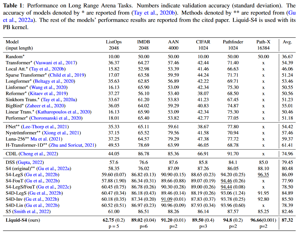
Tested on the LRA, this approach appears to be the best. Only Mega, published few days earlier and therefore not present in the paper, does better:

Figure 16: Liquid-S4 results on the LRA benchmark

HASANI, LECHNER et al. also apply their model to the Speech Commands, sCIFAR and BIDMC Vital Signs datasets of PIMENTEL et al. and establish the new state of the art.

To dig deeper
The official implementation is available on GitHub.
Exchanges on Open Review.
The official LTC implementation is available on GitHub.

S5: Simplified State Space Layers for Sequence Modeling

Chronologically, the Simplified State Space Layers for Sequence Modeling by SMITH, WARRINGTON and LINDERMAN introducing the S5 model was unveiled on August 9, 2022, so before the Mega and Liquid-S5. However, I'm tackling this paper after the latter because on October 6, 2022, the authors of the S5 updated their publication, improving their model by more than 5 points on the LRA compared with V1. What's more, they propose a comparison covering all SSMs released in 2022. It seemed to me more appropriate to approach S5 from its V2.

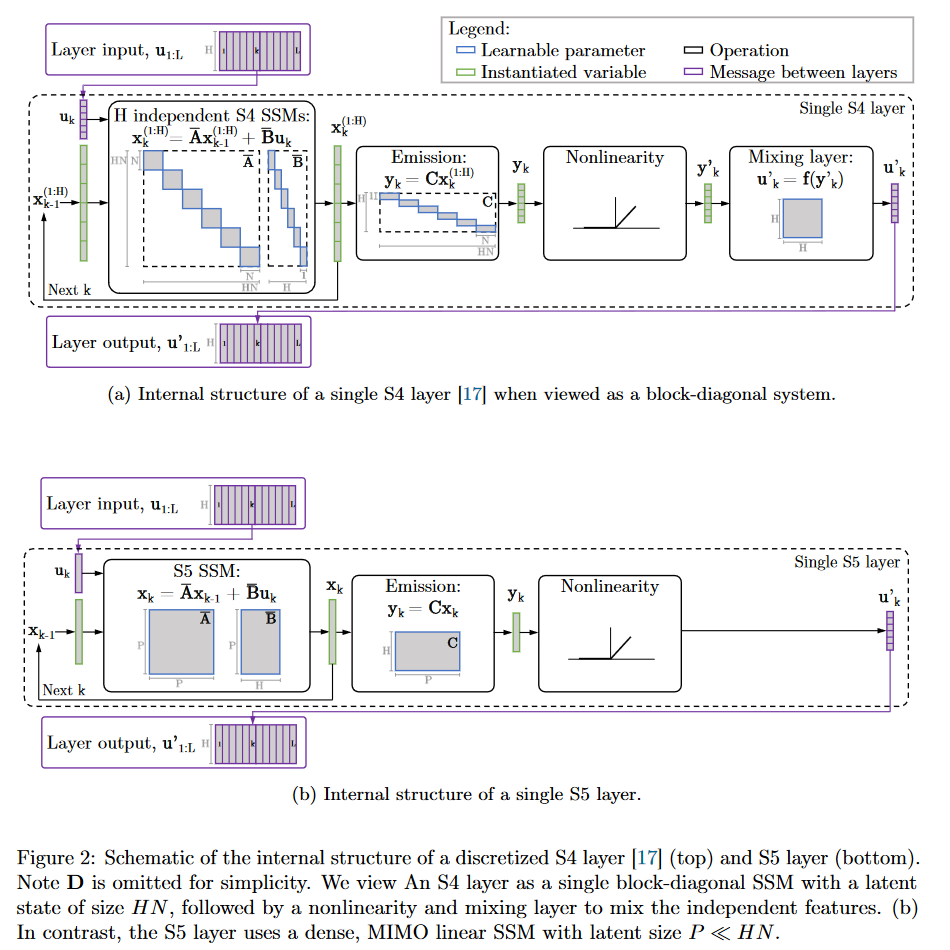
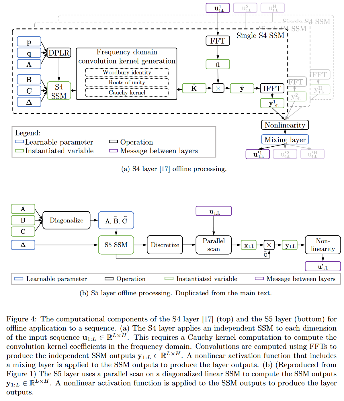
In S5, the authors propose to replace the formulation of S4 using a bank of independent single-input/single-output (SISO) SSMs with a multi-input/multi-output (MIMO) SSM, which has a reduced latent dimension.

Figure 17: S4 vs. S5 internal behavior

The reduced latent dimension of the MIMO system allows the use of the parallel scan algorithm, which simplifies the calculations required to apply the S5 layer as a sequence-to-sequence transformation. The resulting model thus loses the convolutional view of the SSM and focuses solely on the recurrent view (obtained by ZOH discretization). The authors' approach is therefore to operate in the time domain rather than the frequency domain. They use a diagonal approximation of the HiPPO matrix, enabling efficient initialization and parameterization for their MIMO system.

Figure 19: Full comparison of S4 vs. S5 behaviour

As the use of parallel scan is a component used in other SSMs in the future (notably Mamba), let's take a closer look at how it works in S5, so as to familiarize ourselves with this algorithm right from this article. The easiest way to do this is to use the example given in appendix H of the paper, where the authors apply it to a sequence of length $L=4L\; =\; 4$.

To calculate a parallel scan, two things are required:

• The initial elements on which the scan will operate.
  We define the initial elements of a sequence of length $LL$ as, $c_{1:L}c\_\{1:L\}$, so that each element $c_{k}c\_k$ is the tuple $c_k=(c_{k,a},c_{k,b}):=(\bar{\mathbf{A}},\bar{\mathbf{B}}{u}_k)c\_k\; =\; (c\_\{k,a\},\; c\_\{k,b\})\; :=\; (\backslash overline\{\backslash mathbf\{A\}\},\backslash enspace\; \backslash overline\{\backslash mathbf\{B\}\}u\_k)$. In the case of $L=4L\; =\; 4$, we therefore have $(\bar{\mathbf{A}},\bar{\mathbf{B}}{u}_1),(\bar{\mathbf{A}},\bar{\mathbf{B}}{u}_2),(\bar{\mathbf{A}},\bar{\mathbf{B}}{u}_3)(\backslash overline\{\backslash mathbf\{A\}\},\backslash enspace\; \backslash overline\{\backslash mathbf\{B\}\}u\_1),\; (\backslash overline\{\backslash mathbf\{A\}\},\; \backslash enspace\; \backslash overline\{\backslash mathbf\{B\}\}u\_2),(\backslash overline\{\backslash mathbf\{A\}\},\backslash enspace\; \backslash overline\{\backslash mathbf\{B\}\}u\_3)$ and $(\bar{\mathbf{A}},\bar{\mathbf{B}}{u}_4)(\backslash overline\{\backslash mathbf\{A\}\},\backslash enspace\; \backslash overline\{\backslash mathbf\{B\}\}u\_4)$.
• A binary associative operator used to combine elements. Mathematically, a binary associative operator is $I\bullet J\bullet K=(I\bullet J)\bullet K=I\bullet (J\bullet K)I\; \backslash bullet\; J\; \backslash bullet\; K\; =\; (I\; \backslash bullet\; J)\backslash bullet\; K\; =\; I\; \backslash bullet\; (J\; \backslash bullet\; K)$.

If we were to proceed sequentially with the scan, posing $s_0:=(\mathbf{I},0)s\_0:=(\backslash mathbf\{I\},0)$, we would have to perform 4 calculations to obtain the 4 outputs $s_{i}s\_i$ :
$s_1=s_0\bullet c_1=(\mathbf{I},0)\bullet (\bar{\mathbf{A}},\bar{\mathbf{B}}{u}_1)=(\bar{\mathbf{A}}\mathbf{I},\bar{\mathbf{A}}0+\bar{\mathbf{B}}{u}_1)=(\bar{\mathbf{A}},\bar{\mathbf{B}}{u}_1)s\_1\; =\; s\_0\; \backslash bullet\; c\_1\; =\; (\backslash mathbf\{I\},\backslash enspace\; 0)\; \backslash bullet\; (\backslash overline\{\backslash mathbf\{A\}\},\backslash enspace\; \backslash overline\{\backslash mathbf\{B\}\}u\_1)\; =\; (\backslash overline\{\backslash mathbf\{A\}\}\backslash mathbf\{I\},\backslash enspace\; \backslash overline\{\backslash mathbf\{A\}\}0+\backslash overline\{\backslash mathbf\{B\}\}u\_1)\; =\; (\backslash overline\{\backslash mathbf\{A\}\},\backslash enspace\; \backslash overline\{\backslash mathbf\{B\}\}u\_1)$
$s_2=s_1\bullet c_2=(\bar{\mathbf{A}},\bar{\mathbf{B}}{u}_1)\bullet (\bar{\mathbf{A}},\bar{\mathbf{B}}{u}_2)=({\bar{\mathbf{A}}}^2,\bar{\mathbf{A}}\bar{\mathbf{B}}{u}_1+\bar{\mathbf{B}}{u}_2)s\_2\; =\; s\_1\; \backslash bullet\; c\_2\; =(\backslash overline\{\backslash mathbf\{A\}\},\backslash enspace\; \backslash overline\{\backslash mathbf\{B\}\}u\_1)\; \backslash bullet\; (\backslash overline\{\backslash mathbf\{A\}\},\backslash enspace\; \backslash overline\{\backslash mathbf\{B\}\}u\_2)\; =\; (\backslash overline\{\backslash mathbf\{A\}\}^2,\backslash enspace\; \backslash overline\{\backslash mathbf\{A\}\}\backslash overline\{\backslash mathbf\{B\}\}u\_1\; +\; \backslash overline\{\backslash mathbf\{B\}\}u\_2\; )$
$s_3=s_2\bullet c_3=({\bar{\mathbf{A}}}^2,\bar{\mathbf{A}}\bar{\mathbf{B}}{u}_1+\bar{\mathbf{B}}{u}_2)\bullet (\bar{\mathbf{A}},\bar{\mathbf{B}}{u}_3)=({\bar{\mathbf{A}}}^3,{\bar{\mathbf{A}}}^2\bar{\mathbf{B}}{u}_1+\bar{\mathbf{A}}\bar{\mathbf{B}}{u}_2+\bar{\mathbf{B}}{u}_3)s\_3\; =\; s\_2\; \backslash bullet\; c\_3\; =\; (\backslash overline\{\backslash mathbf\{A\}\}^2,\backslash enspace\; \backslash overline\{\backslash mathbf\{A\}\}\backslash overline\{\backslash mathbf\{B\}\}u\_1\; +\; \backslash overline\{\backslash mathbf\{B\}\}u\_2\; )\; \backslash bullet\; (\backslash overline\{\backslash mathbf\{A\}\},\backslash enspace\; \backslash overline\{\backslash mathbf\{B\}\}u\_3)\; =\; (\backslash overline\{\backslash mathbf\{A\}\}^3,\backslash enspace\; \backslash overline\{\backslash mathbf\{A\}\}^2\backslash overline\{\backslash mathbf\{B\}\}u\_1\; +\; \backslash overline\{\backslash mathbf\{A\}\}\backslash overline\{\backslash mathbf\{B\}\}u\_2\; +\; \backslash overline\{\backslash mathbf\{B\}\}u\_3)$
$s_4=s_3\bullet c_4=({\bar{\mathbf{A}}}^3,{\bar{\mathbf{A}}}^2\bar{\mathbf{B}}{u}_1+\bar{\mathbf{A}}\bar{\mathbf{B}}{u}_2+\bar{\mathbf{B}}{u}_3)\bullet (\bar{\mathbf{A}},\bar{\mathbf{B}}{u}_4)=({\bar{\mathbf{A}}}^4,{\bar{\mathbf{A}}}^3\bar{\mathbf{B}}{u}_1+{\bar{\mathbf{A}}}^2\bar{\mathbf{B}}{u}_2+\bar{\mathbf{A}}\bar{\mathbf{B}}{u}_3+\bar{\mathbf{B}}{u}_4)\mathrm{.}s\_4\; =\; s\_3\; \backslash bullet\; c\_4\; =\; (\backslash overline\{\backslash mathbf\{A\}\}^3,\backslash enspace\; \backslash overline\{\backslash mathbf\{A\}\}^2\backslash overline\{\backslash mathbf\{B\}\}u\_1\; +\; \backslash overline\{\backslash mathbf\{A\}\}\backslash overline\{\backslash mathbf\{B\}\}u\_2\; +\; \backslash overline\{\backslash mathbf\{B\}\}u\_3)\; \backslash bullet\; (\backslash overline\{\backslash mathbf\{A\}\},\backslash enspace\; \backslash overline\{\backslash mathbf\{B\}\}u\_4)\backslash \backslash \; =\; (\backslash overline\{\backslash mathbf\{A\}\}^4,\; \backslash enspace\; \backslash overline\{\backslash mathbf\{A\}\}^3\backslash overline\{\backslash mathbf\{B\}\}u\_1\; +\; \backslash overline\{\backslash mathbf\{A\}\}^2\backslash overline\{\backslash mathbf\{B\}\}u\_2\; +\; \backslash overline\{\backslash mathbf\{A\}\}\backslash overline\{\backslash mathbf\{B\}\}u\_3\; +\; \backslash overline\{\backslash mathbf\{B\}\}u\_4).$

To obtain the $x_{i}x\_i$ states, we would then have to take the second element of each $s_{i}s\_i$ tuple.

Proceeding sequentially is not the most efficient way, since it is possible to parallelize the calculation of a recurrence with parallel scan. Here's an illustration of how it works with our sequence of size $LL$ = 4 :

Figure 19: How parallel scan works in S5

Again, to obtain the $x_{i}x\_i$ states, we'd have to take the second element of each $s_{i}s\_i$ tuple.
You'll notice here that it's possible to calculate $s_{2}s\_2$ and $i_{4}i\_4$ in parallel, then $s_{1}s\_1$, $s_{3}s\_3$ and $s_{4}s\_4$ in parallel. This reduces the number of sequential calculations from 4 to just 2. The complexity of the parallel scan is $O(log(L))O(log(L))$.

Figure 20: How parallel scan works in general. Based on the animation by Scott Linderman.

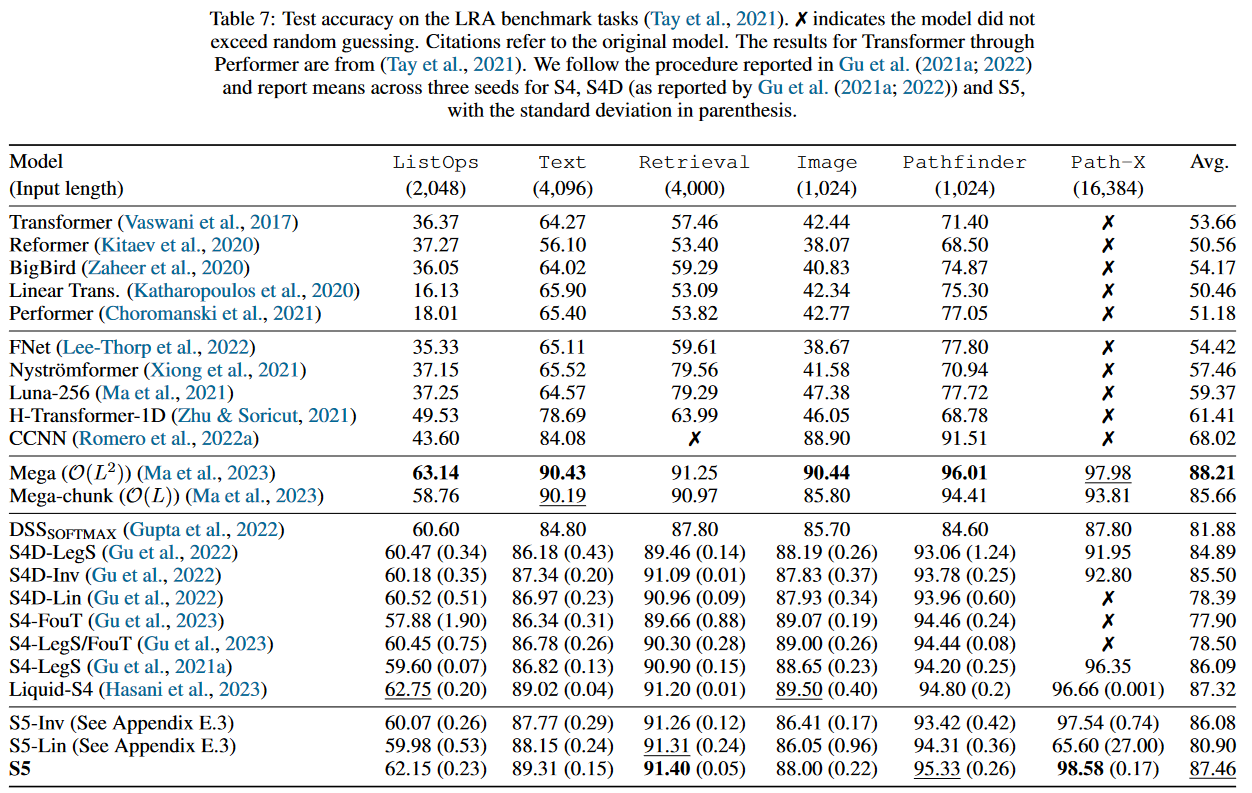
In terms of performance, the S5 ranks second on the LRA :

Figure 21: S5 results on the LRA benchmark

In addition to the LRA, the authors of S5 compare their model on the Speech Commands, the pendulum regression dataset as well as sMNIST, psMNIST and sCIFAR. The full results are available in the paper's appendix, which also contains an ablation study.

To dig deeper
The official implementation is available on GitHub.
Exchanges on Open Review.

SGConv

On October 17, 2022, What Makes Convolutional Models Great on Long Sequence Modeling? LI, CAI et al. report that they find S4 too complex, requiring sophisticated parameterization and initialization schemes (= HiPPO). And consequently that it is less intuitive and difficult to use for people with limited prior knowledge. So their aim is to demystify S4 by focusing on its convolutional view. They identify two critical principles from which S4 benefits and which are sufficient to constitute a high-performance global convolutional model:

1. The parameterization of the convolutional kernel must be efficient in the sense that the number of parameters must increase sub-linearly with sequence length.
2. The kernel must have a decreasing structure in which the weights for convolution with the nearest neighbors are greater than those for the farthest neighbors.

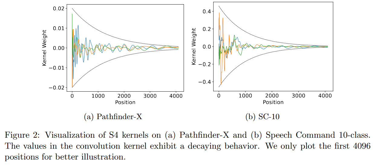Figure 22: Respecting the two critical principles set out by the authors means having convolution kernels resembling those shown in the figure.

Based on these two principles, they propose an efficient convolutional model called Structured Global Convolution (SGConv).

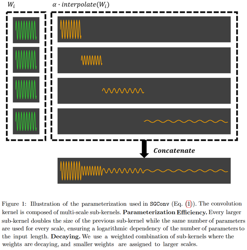Figure 23: SGConv constructs convolution kernels as the concatenation of successively longer sinusoids of lower norm. The advantage of this form is that it enables very fast convolution in the frequency domain.

The SGConv authors report better results than the S4 on several tasks (text, audio, image). We won't go into detail here. Let's just look at the LRA:

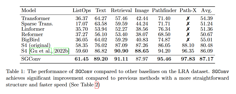Figure 24: SGConv results on LRA.

Indeed, looking at this table, we can see that the SGConv does better than both versions of the S4. Nevertheless, it's curious that the authors don't include the Mega, Liquid-S4 or S5 in their comparison, which all achieve better results using a convolution kernel that is a sum of decreasing exponential functions.
What's more, while all the models evaluated on the LRA treat data as 1D sequences, SGConv implicitly incorporates a 2D inductive bias for image tasks, including PathX, which is questionable.

In the end, SGConv seems to perform similarly to the most recent SSM variants, but loses the recurrent view of S4.
Nevertheless, this paper appears to be the first to focus solely on the convolutional view of an SSM.

To dig deeper
The official implementation is available on GitHub.
Exchanges on Open Review.

Other models

Two other "theoretical" papers were published in 2022. The Pretraining Without Attention by WANG et al. introducing BiGS and the Hungry Hungry Hippos: Towards Language Modeling with State Space Models by FU, DAO et al. introducing H3.
Due to their late publication (December 20 and 28, 2022 respectively) and their communication made in 2023 after the V2s of each of these papers, I will deal with these models in the next article in the SSM series.

SSM applications

SaShiMi

In It's Raw! Audio Generation with State-Space Models published on February 20, 2022, GOEL, GU et al. apply S4 to causal audio generation.
In contrast to methods based on conditioning from texts, spectrograms, etc., this is a method that operates directly on the input signal, enabling comparisons with WaveNet by OORD et al. (2016).
SaShiMi can train directly on sequences of over 100K (8s audio) on a single V100 GPU, compared to the context length limitations faced by models like WaveNet. It makes effective use of this long context to improve density estimation.
The authors have compared their model on various benchmarks including piano music generation and speech (enunciation of numbers).
The generated audios can be viewed here.

Figure 25: Sashimi architecture overview

To dig deeper
The official implementation is available on GitHub.

ViS4mer

On April 4, 2022, ISLAM and BERTASIUS introduce the ViS4mer in their Long Movie Clip Classification with State-Space Video Models.
It's a hybrid between an S4 and a Transformer for (long) video classification. More precisely, the model uses a standard Transformer encoder for short-range spatiotemporal feature extraction, and a multi-scale temporal S4 decoder for long-range temporal reasoning. The resulting model appears to be 2.6 times faster and 8 times more memory-efficient than a Transformer.
To my knowledge, this is the first paper to highlight the benefits of hybridizing SSMs and Transformers.

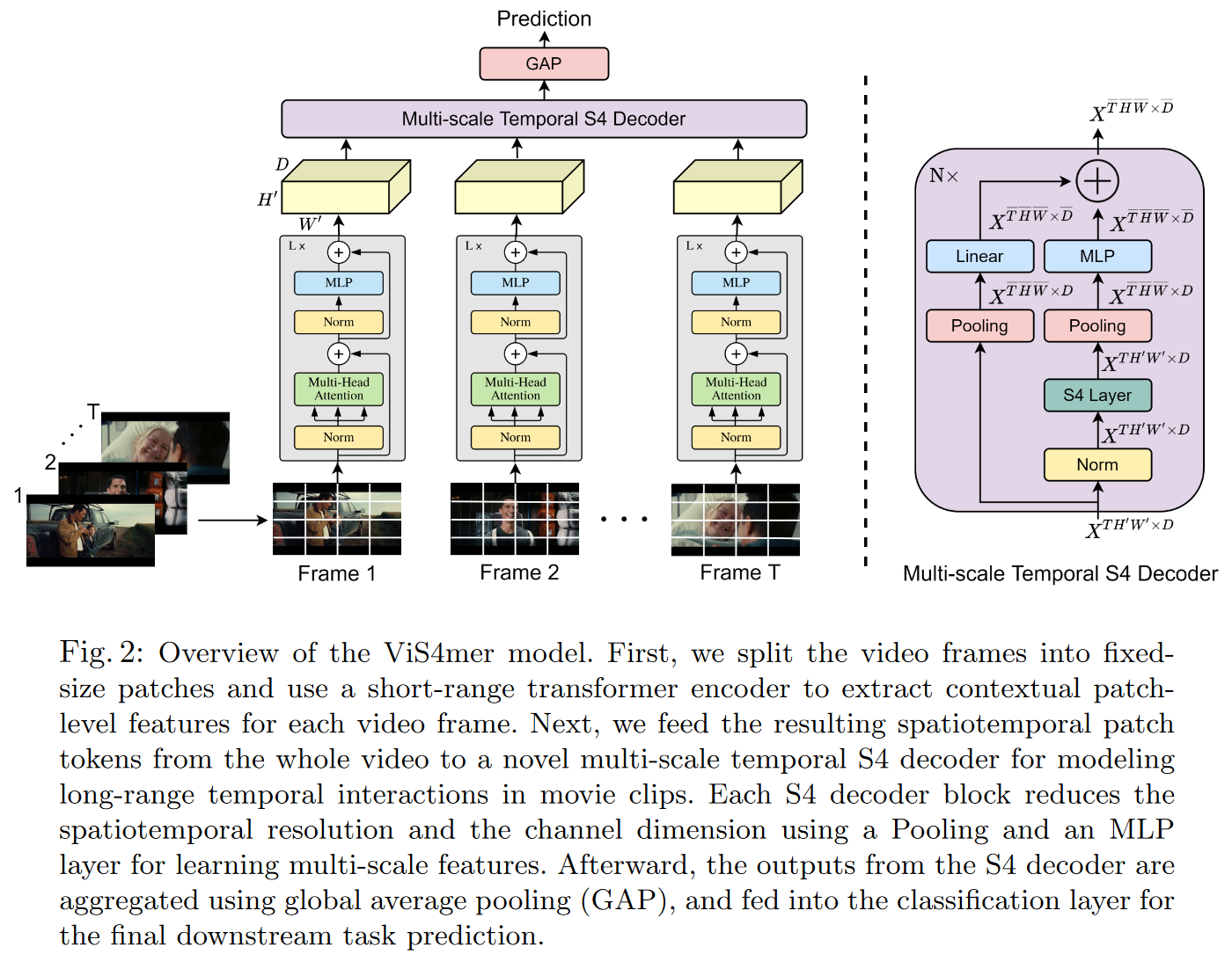Figure 26: ViS4mer decoder overview

ViS4mer achieves top results in 6 out of 9 long video classification tasks on the benchmark Long Video Understanding (LVU) by WU and KRÄHENBÜHL (2021), which consists of classifying videos with a duration of 1 to 3 min. The model also appears to have good generalization capabilities, achieving competitive results on the Breakfast and COIN procedural activity datasets despite having seen 275 times less data.

To dig deeper
The official implementation is available on GitHub.

CCNN

On June 7, 2022, ROMERO, KNIGGE et al. introduced CCNN in their paper Towards a General Purpose CNN for Long Range Dependencies in ND.
Their starting point is the idea that convolutional neural networks are powerful but need to be adapted specifically to each task:

• Input length: 32x32, 1024x1024 → How to model long-range dependencies?
• Input resolution: 8kHz, 16kHz → Long-range dependencies, resolution agnosticity?
• Input dimensionality: 1D, 2D, 3D → How to define convolutional kernels?
• Task: Classification, Segmentation, ... → How to define high-low sampling strategies?
  Is it then possible to design a unique architecture, with which tasks can be solved independently of dimensionality, resolution and input length, without modifying the architecture? Yes, thanks to CCNN, which uses continuous convolution kernels.

ROMERO, KNIGGE et al. drew inspiration from the S4 to create a variant of efficient residual blocks, which they call S4 block. However, unlike the S4, which only works with 1D signals, the CCNN easily models ND signals.

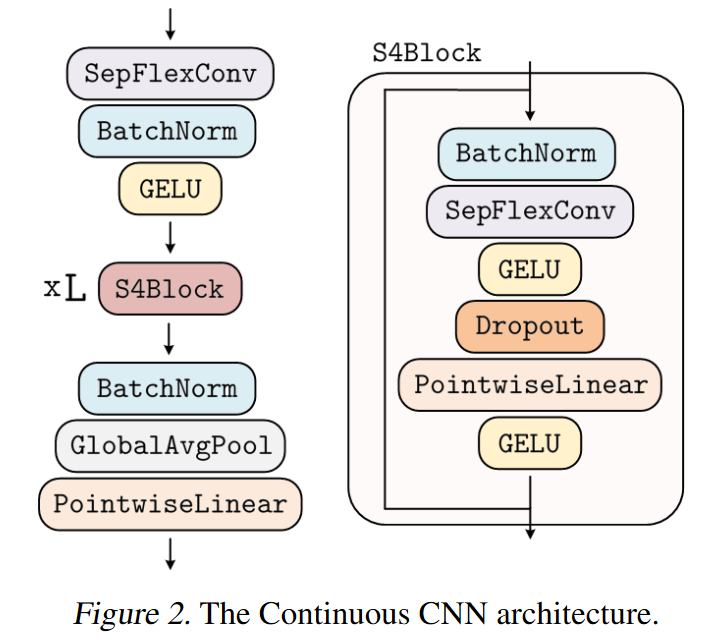Figure 27: Overview of CCNN

To dig deeper
The official implementation is available on GitHub.
Slides from a presentation of the paper are available here

$\mathbf{S}\mathbf{S}\mathbf{S}{\mathbf{D}}^{\mathbf{S}\mathbf{4}}\backslash mathbf\{SSSD^\{S4\}\}$

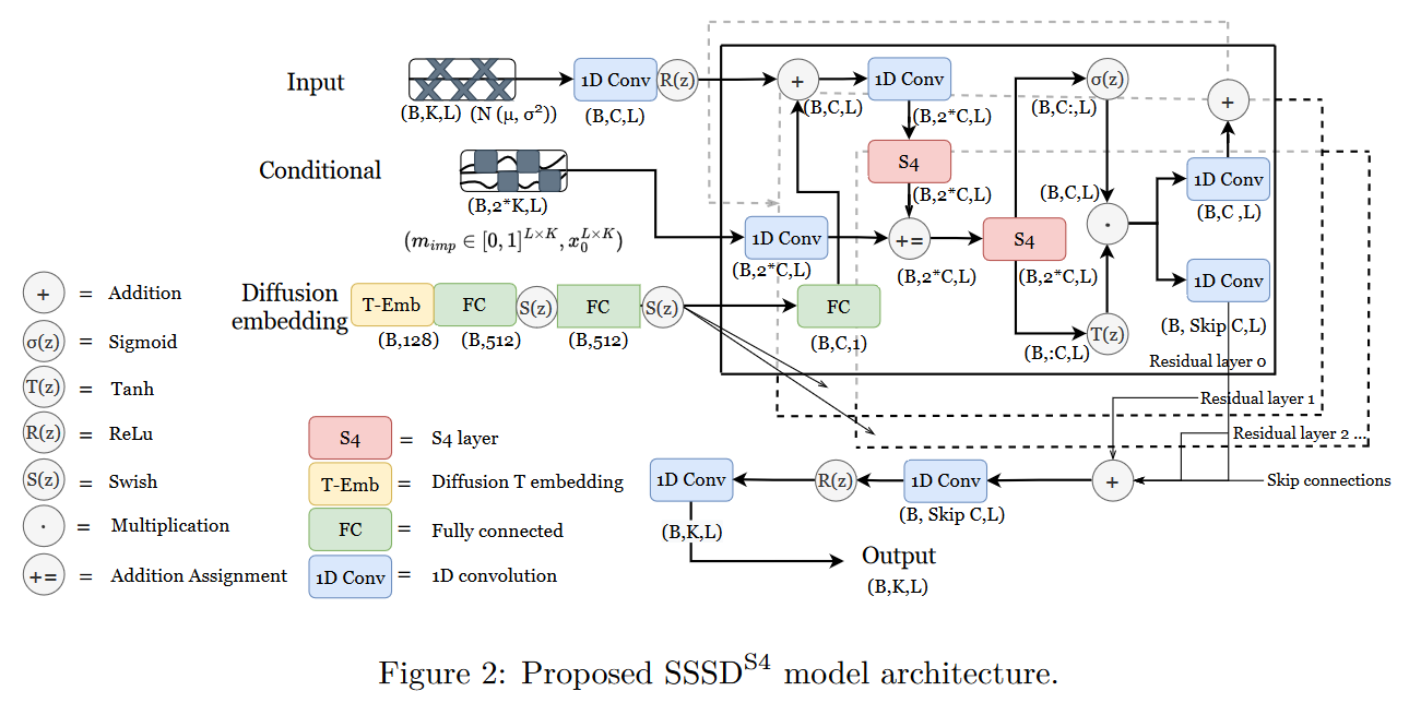
On August 19, 2022, LOPEZ ALCARAZ and STRODTHOFF proposed in their paper Diffusion-based Time Series Imputation and Forecasting with Structured State Space Models a hybrid between an S4 and a diffusion model for predicting missing data in time series. Their model is called $\mathbf{S}\mathbf{S}\mathbf{S}{\mathbf{D}}^{\mathbf{S}\mathbf{4}}\backslash mathbf\{SSSD^\{S4\}\}$ (or simply SSSD).

Figure 28: SSSD overview

To dig deeper
The official implementation is available on GitHub.

S4ND

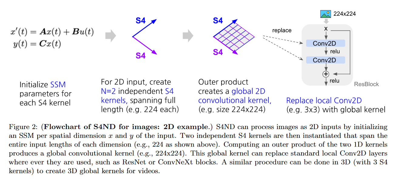
On October 12, 2022, NGUYEN, GOEL, GU et al. present S4ND: Modeling Images and Videos as Multidimensional Signals Using State Spaces.

This model extends S4 (which is 1D) to multidimensional continuous signals such as images and videos (where ConvNets and ViT learn on discrete pixels). To do this, they transform the standard S4 ODE into a multidimensional PDE:

becomes :

with ${\mathbf{A}}^{(\tau )}\in {\mathbb{C}}^{N^{(\tau )}\times N^{(\tau )}}\backslash mathbf\{A\}^\{(\backslash tau)\}\; \backslash in\; \backslash mathbb\{C\}^\{N^\{(\backslash tau)\}\; \backslash times\; N^\{(\backslash tau)\}\}$, ${\mathbf{B}}^{(\tau )}\in {\mathbb{C}}^{N^{(\tau )}\times 1}\backslash mathbf\{B\}^\{(\backslash tau)\}\; \backslash in\; \backslash mathbb\{C\}^\{N^\{(\backslash tau)\}\; \backslash times\; 1\}$, $\mathbf{C}\in {\mathbb{C}}^{N^{(1)}\times N^{(2)}}\backslash mathbf\{C\}\; \backslash in\; \backslash mathbb\{C\}^\{N^\{(1)\}\; \backslash times\; N^\{(2)\}\}$, with the initial condition of the linear PDE $x(0,0)=0x(0,\; 0)\; =\; 0$.

Depending on the dataset tested, the authors obtain results similar to or better than those of ViT or ConvNext.
The main advantage of S4ND is that it can operate at different resolutions via different sampling rates. The authors highlight this feature in two experiments:

1. In zero-shot, S4ND outperforms Conv2D by more than 40 points when trained on $8\times 88\backslash times8$ images and tested on $32\times 3232\backslash times32$ images.
2. With progressive resizing, S4ND can speed up training by 22% with a decrease in final accuracy of ∼1% compared to training at high resolution alone.

Figure 30: Example of S4ND for 2D images

To dig deeper
The official implementation is available on GitHub.
A completely useless but amusing piece of information: the authors have called their TeX file Darude S4NDstorm.

Conclusion

We therefore reviewed the various SSM models released in 2022. This was a year in which work focused mainly on improving/simplifying S4 via various approaches (diagonalization, gating, LTC, etc.). The year 2022 also saw the first applications of SSM.
With SGConv and S5, we can also see the beginnings of a phenomenon which, as we'll see in the following article, will become more pronounced in 2023. Namely, the emergence of works focusing solely on the convolutional view of SSMs (e.g. Hyena and its derivatives) or focusing solely on the recursive view of SSMs (e.g. Mamba).

References

• Combining Recurrent, Convolutional, and Continuous-time Models with Linear State-Space Layers d'Albert GU, Isys JOHNSON, Karan GOEL, Khaled SAAB, Tri DAO, Atri RUDRA, Christopher RÉ (2021)
• Efficiently Modeling Long Sequences with Structured State Spaces d'Albert GU, Karan GOEL, et Christopher RÉ (2021)
• HiPPO: Recurrent Memory with Optimal Polynomial Projections d'Albert GU, Tri DAO, Stefano ERMON, Atri RUDRA, Christopher RÉ (2020)
• How to Train Your HiPPO d'Albert GU, Isys JOHNSON, Aman TIMALSINA, Atri RUDRA, and Christopher RÉ (2022)
• Long Range Arena: A Benchmark for Efficient Transformers de Yi TAY, Mostafa DEHGHANI, Samira ABNAR, Yikang SHEN, Dara BAHRI, Philip PHAM, Jinfeng RAO, Liu YANG, Sebastian RUDER et Donald METZLER (2020)
• Diagonal State Spaces are as Effective as Structured State Spaces de Ankit GUPTA, Albert GU et Jonathan BERANT (2022)
• Speech Commands: A Dataset for Limited-Vocabulary Speech Recognition de Pete WARDEN (2018)
• Simplifying and Understanding State Space Models with Diagonal Linear RNNs de Ankit GUPTA, Harsh MEHTA et Jonathan BERANT (2022)
• On the Parameterization and Initialization of Diagonal State Space Models d'Albert GU, Ankit GUPTA, Karan GOEL, Christopher RÉ
• Long Range Language Modeling via Gated State Spaces d'Harsh MEHTA, Ankit GUPTA, Ashok CUTKOSKY et Behnam NEYSHABUR (2022)
• Language Modeling with Gated Convolutional Networks de Yann N. DAUPHIN, Angela FAN, Michael AULI et David GRANGIER (2016)
• GLU Variants Improve Transformer de Noam SHAZEER (2020)
• Transformer Quality in Linear Time de Weizhe HUA, Zihang DAI, Hanxiao LIU et Quoc V. LE (2022)
• Mega: Moving Average Equipped Gated Attention de Xuezhe MA, Chunting ZHOU, Xiang KONG, Junxian HE, Liangke GUI, Graham NEUBIG, Jonathan MAY et Luke ZETTLEMOYER (2022)
• Liquid Structural State-Space Models de Ramin HASANI, Mathias LECHNER, Tsun-Hsuan WANG, Makram CHACHINE, Alexander AMINI et Daniela RUS (2022)
• Liquid Time-constant Networks de Ramin HASANI, Mathias LECHNER, Alexander AMINI, Daniela RUS et Radu GROSU (2021)
• Simplified State Space Layers for Sequence Modeling de Jimmy T.H. SMITH, Andrew WARRINGTON et Scott W. LINDERMAN (2022)
• Toward a Robust Estimation of Respiratory Rate From Pulse Oximeters de Marco A. F. PIMENTEL, Alistair E. W. JOHNSON, Peter H. CHARLTON, Drew BIRRENKOTT, Peter J. WATKINSON, Lionel TARASSENKO et David A. CLIFTON (2017)
• What Makes Convolutional Models Great on Long Sequence Modeling? de Yuhong LI, Tianle CAI, Yi ZHANG, Deming CHEN et Debadeepta DEY (2022)
• Pretraining Without Attention de Junxiong WANG, Jing Nathan YAN, Albert GU et Alexander M. RUSH (2022)
• Hungry Hungry Hippos: Towards Language Modeling with State Space Models de Daniel Y. FU, Tri DAO, Khaled K. SAAB, Armin W. THOMAS, Atri RUDRA et Christopher RÉ (2022)
• It's Raw! Audio Generation with State-Space Models de Karan GOEL, Albert GU, Chris DONAHUE, Christopher RÉ (2022)
• WaveNet: A Generative Model for Raw Audio de Aaron van den OORD, Sander DIELEMAN, Heiga ZEN, Karen SIMONYAN, Oriol VINYALS, Alex GRAVES, Nal KALCHBRENNER, Andrew SENIOR et Koray KAVUKCCUOGLU
• Long Movie Clip Classification with State-Space Video Models de Md Mohaiminul ISLAM, Gedas BERTASIUS (2022)
• Long Video Understanding de Chao-Yuan WU et Philipp KRÄHENBÜHL (2021)
• Towards a General Purpose CNN for Long Range Dependencies in ND de David W. ROMERO, David M. KNIGGE, Albert GU, Erik J. BEKKERS, Efstratios GAVVES, Jakub M. TOMCZAK, Mark HOOGENDOORN (2022)
• Diffusion-based Time Series Imputation and Forecasting with Structured State Space Models de Juan Miguel LOPEZ ALCARAZ, Nils STRODTHOFF (2022)
• S4ND: Modeling Images and Videos as Multidimensional Signals Using State Spaces de Eric NGUYEN, Karan GOEL, Albert GU, Gordon W. DOWNS, Preey SHAH, Tri DAO, Stephen A. BACCUS, Christopher RÉ (2022)
  
  
  

Citation

@inproceedings{ssm_in_2022_blog_post,
author = {Loïck BOURDOIS},
title = {Évolution des State Space Models (SSM) en 2022},
year = {2023},
url = {https://lbourdois.github.io/blog/ssm/ssm_en_2022}
}